Free Statistics
of Irreproducible Research!
Description of Statistical Computation | |||||||||||||||||||||
|---|---|---|---|---|---|---|---|---|---|---|---|---|---|---|---|---|---|---|---|---|---|
| Author's title | |||||||||||||||||||||
| Author | *The author of this computation has been verified* | ||||||||||||||||||||
| R Software Module | rwasp_meanplot.wasp | ||||||||||||||||||||
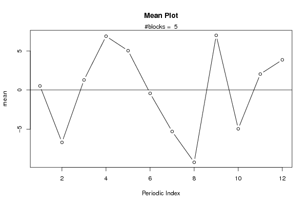
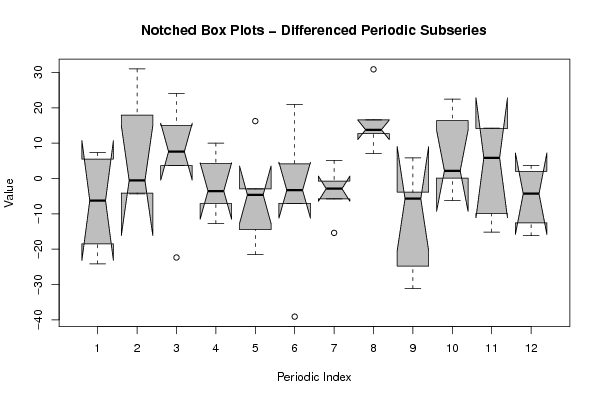
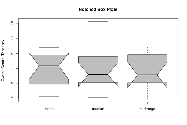
| Title produced by software | Mean Plot | ||||||||||||||||||||
| Date of computation | Mon, 09 Nov 2009 06:49:06 -0700 | ||||||||||||||||||||
| Cite this page as follows | Statistical Computations at FreeStatistics.org, Office for Research Development and Education, URL https://freestatistics.org/blog/index.php?v=date/2009/Nov/09/t125777459591xi1almaliq91l.htm/, Retrieved Fri, 19 Apr 2024 14:04:33 +0000 | ||||||||||||||||||||
| Statistical Computations at FreeStatistics.org, Office for Research Development and Education, URL https://freestatistics.org/blog/index.php?pk=54820, Retrieved Fri, 19 Apr 2024 14:04:33 +0000 | |||||||||||||||||||||
| QR Codes: | |||||||||||||||||||||
|
| |||||||||||||||||||||
| Original text written by user: | |||||||||||||||||||||
| IsPrivate? | No (this computation is public) | ||||||||||||||||||||
| User-defined keywords | |||||||||||||||||||||
| Estimated Impact | 150 | ||||||||||||||||||||
Tree of Dependent Computations | |||||||||||||||||||||
| Family? (F = Feedback message, R = changed R code, M = changed R Module, P = changed Parameters, D = changed Data) | |||||||||||||||||||||
| - [Box-Cox Linearity Plot] [3/11/2009] [2009-11-02 21:47:57] [b98453cac15ba1066b407e146608df68] - RMPD [Mean Plot] [] [2009-11-09 13:49:06] [9f6463b67b1eb7bae5c03a796abf0348] [Current] | |||||||||||||||||||||
| Feedback Forum | |||||||||||||||||||||
Post a new message | |||||||||||||||||||||
Dataset | |||||||||||||||||||||
| Dataseries X: | |||||||||||||||||||||
-9.689129094 -15.9156891 -20.03555923 -12.44264761 -2.468740667 -23.97386436 -3.02331487 -8.793616067 3.890809296 -1.836563963 -1.709285854 4.14432084 -12.03301028 -4.733406668 -5.29923341 -1.665398243 2.528592702 -2.076860346 2.08284686 1.362751533 17.9705551 -13.16742762 9.297539752 -0.631604907 -9.595566233 -4.093437696 -8.465289457 15.56005027 8.440539387 5.496633362 -1.542161774 -4.424920628 9.358249829 5.491823987 21.87928431 6.722498409 7.093000066 -17.05020325 0.883582789 15.92450566 3.185445132 -11.26933787 -14.58358037 -29.97174154 0.914837609 6.714446914 8.903871839 23.13841004 26.84332477 8.351341468 39.34532234 16.99485377 13.45289299 29.686769 -9.403389414 -4.311467414 2.792229304 -21.98399447 -28.17586045 -14.08502665 | |||||||||||||||||||||
Tables (Output of Computation) | |||||||||||||||||||||
| |||||||||||||||||||||
Figures (Output of Computation) | |||||||||||||||||||||
Input Parameters & R Code | |||||||||||||||||||||
| Parameters (Session): | |||||||||||||||||||||
| par1 = 12 ; | |||||||||||||||||||||
| Parameters (R input): | |||||||||||||||||||||
| par1 = 12 ; | |||||||||||||||||||||
| R code (references can be found in the software module): | |||||||||||||||||||||
par1 <- as.numeric(par1) | |||||||||||||||||||||