Free Statistics
of Irreproducible Research!
Description of Statistical Computation | |||||||||||||||||||||
|---|---|---|---|---|---|---|---|---|---|---|---|---|---|---|---|---|---|---|---|---|---|
| Author's title | |||||||||||||||||||||
| Author | *The author of this computation has been verified* | ||||||||||||||||||||
| R Software Module | rwasp_cloud.wasp | ||||||||||||||||||||
| Title produced by software | Trivariate Scatterplots | ||||||||||||||||||||
| Date of computation | Mon, 09 Nov 2009 05:59:13 -0700 | ||||||||||||||||||||
| Cite this page as follows | Statistical Computations at FreeStatistics.org, Office for Research Development and Education, URL https://freestatistics.org/blog/index.php?v=date/2009/Nov/09/t1257771633z36smjrpglt3d7d.htm/, Retrieved Sat, 20 Apr 2024 08:02:02 +0000 | ||||||||||||||||||||
| Statistical Computations at FreeStatistics.org, Office for Research Development and Education, URL https://freestatistics.org/blog/index.php?pk=54793, Retrieved Sat, 20 Apr 2024 08:02:02 +0000 | |||||||||||||||||||||
| QR Codes: | |||||||||||||||||||||
|
| |||||||||||||||||||||
| Original text written by user: | |||||||||||||||||||||
| IsPrivate? | No (this computation is public) | ||||||||||||||||||||
| User-defined keywords | WS5 trivariate | ||||||||||||||||||||
| Estimated Impact | 222 | ||||||||||||||||||||
Tree of Dependent Computations | |||||||||||||||||||||
| Family? (F = Feedback message, R = changed R code, M = changed R Module, P = changed Parameters, D = changed Data) | |||||||||||||||||||||
| - [Trivariate Scatterplots] [WS5 trivariate] [2009-11-09 12:59:13] [b4ff140915b3f24d4faed3d78f95eba4] [Current] - RMP [Partial Correlation] [WS5 parti�le corr...] [2009-11-09 19:36:40] [c620fe7250af73a91c51407172a85dab] - RMPD [Bivariate Explorative Data Analysis] [WS5 bivariate EDA] [2009-11-09 20:25:50] [c620fe7250af73a91c51407172a85dab] - RMPD [Bivariate Explorative Data Analysis] [WS5 bivariate EDA...] [2009-11-09 20:51:38] [c620fe7250af73a91c51407172a85dab] - RMPD [Bivariate Explorative Data Analysis] [WS5 bivariate EDA...] [2009-11-09 21:12:34] [c620fe7250af73a91c51407172a85dab] - RMPD [Bivariate Explorative Data Analysis] [WS5 bivariate eda...] [2009-11-09 21:20:16] [c620fe7250af73a91c51407172a85dab] | |||||||||||||||||||||
| Feedback Forum | |||||||||||||||||||||
Post a new message | |||||||||||||||||||||
Dataset | |||||||||||||||||||||
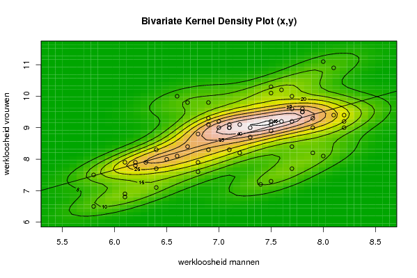
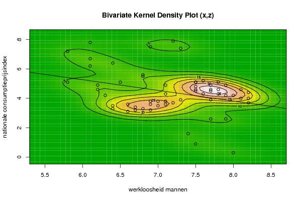
| Dataseries X: | |||||||||||||||||||||
8 8.1 7.7 7.5 7.6 7.8 7.8 7.8 7.5 7.5 7.1 7.5 7.5 7.6 7.7 7.7 7.9 8.1 8.2 8.2 8.2 7.9 7.3 6.9 6.6 6.7 6.9 7 7.1 7.2 7.1 6.9 7 6.8 6.4 6.7 6.6 6.4 6.3 6.2 6.5 6.8 6.8 6.4 6.1 5.8 6.1 7.2 7.3 6.9 6.1 5.8 6.2 7.1 7.7 7.9 7.7 7.4 7.5 8 | |||||||||||||||||||||
| Dataseries Y: | |||||||||||||||||||||
11.1 10.9 10 9.2 9.2 9.5 9.6 9.5 9.1 8.9 9 10.1 10.3 10.2 9.6 9.2 9.3 9.4 9.4 9.2 9 9 9 9.8 10 9.8 9.3 9 9 9.1 9.1 9.1 9.2 8.8 8.3 8.4 8.1 7.7 7.9 7.9 8 7.9 7.6 7.1 6.8 6.5 6.9 8.2 8.7 8.3 7.9 7.5 7.8 8.3 8.4 8.2 7.7 7.2 7.3 8.1 | |||||||||||||||||||||
| Dataseries Z: | |||||||||||||||||||||
4.2 4 4.9 4.6 4.3 4.3 4.6 5.1 4.8 4.5 4.9 5.1 5.1 5.2 4.5 4.6 4.9 4.6 4.4 3.7 4 4.2 3.9 3.6 3.6 3.2 3.2 3.5 3.6 3.7 3.8 3.8 3.8 3.3 3.3 3.4 3.1 3.5 4.2 4.9 5.1 5.5 5.6 6.4 6.2 7.2 7.8 7.9 7.4 7.5 6.7 5.1 4.6 4.3 3.9 2.6 2.6 1.6 0.9 0.3 | |||||||||||||||||||||
Tables (Output of Computation) | |||||||||||||||||||||
| |||||||||||||||||||||
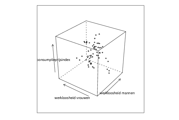
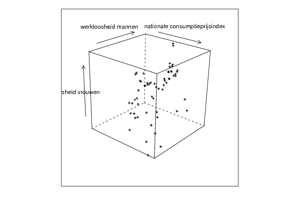
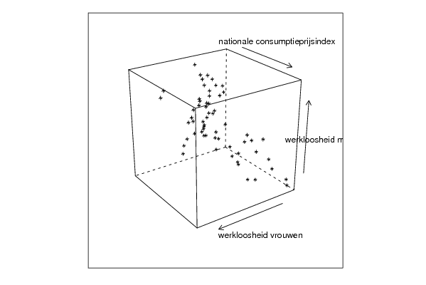
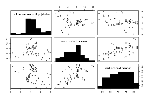
Figures (Output of Computation) | |||||||||||||||||||||
Input Parameters & R Code | |||||||||||||||||||||
| Parameters (Session): | |||||||||||||||||||||
| par1 = 50 ; par2 = 50 ; par3 = Y ; par4 = Y ; par5 = werkloosheid mannen ; par6 = werkloosheid vrouwen ; par7 = nationale consumptieprijsindex ; | |||||||||||||||||||||
| Parameters (R input): | |||||||||||||||||||||
| par1 = 50 ; par2 = 50 ; par3 = Y ; par4 = Y ; par5 = werkloosheid mannen ; par6 = werkloosheid vrouwen ; par7 = nationale consumptieprijsindex ; | |||||||||||||||||||||
| R code (references can be found in the software module): | |||||||||||||||||||||
x <- array(x,dim=c(length(x),1)) | |||||||||||||||||||||