Free Statistics
of Irreproducible Research!
Description of Statistical Computation | |||||||||||||||||||||
|---|---|---|---|---|---|---|---|---|---|---|---|---|---|---|---|---|---|---|---|---|---|
| Author's title | |||||||||||||||||||||
| Author | *The author of this computation has been verified* | ||||||||||||||||||||
| R Software Module | rwasp_sdplot.wasp | ||||||||||||||||||||
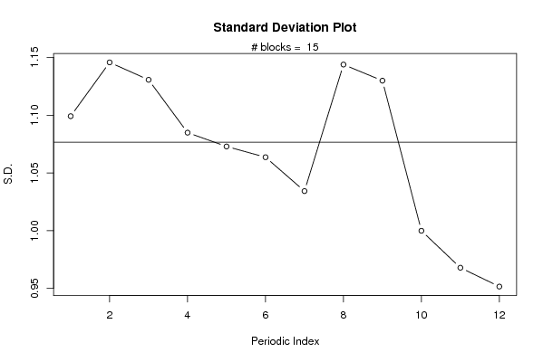
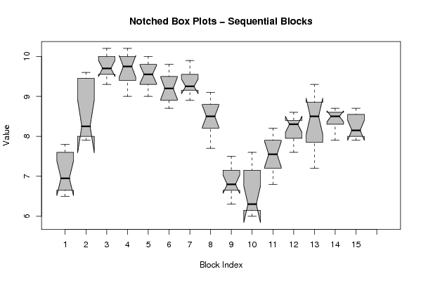
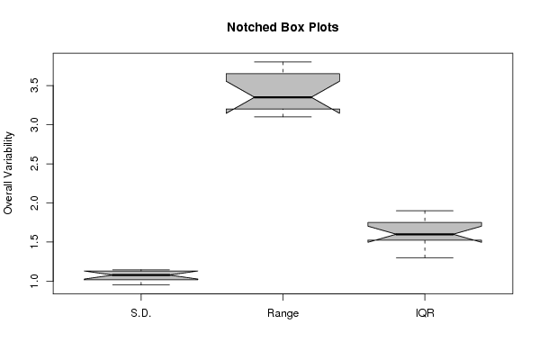
| Title produced by software | Standard Deviation Plot | ||||||||||||||||||||
| Date of computation | Mon, 09 Nov 2009 03:44:27 -0700 | ||||||||||||||||||||
| Cite this page as follows | Statistical Computations at FreeStatistics.org, Office for Research Development and Education, URL https://freestatistics.org/blog/index.php?v=date/2009/Nov/09/t1257763573zlojyt2izr29cq7.htm/, Retrieved Fri, 19 Apr 2024 18:50:32 +0000 | ||||||||||||||||||||
| Statistical Computations at FreeStatistics.org, Office for Research Development and Education, URL https://freestatistics.org/blog/index.php?pk=54720, Retrieved Fri, 19 Apr 2024 18:50:32 +0000 | |||||||||||||||||||||
| QR Codes: | |||||||||||||||||||||
|
| |||||||||||||||||||||
| Original text written by user: | |||||||||||||||||||||
| IsPrivate? | No (this computation is public) | ||||||||||||||||||||
| User-defined keywords | |||||||||||||||||||||
| Estimated Impact | 194 | ||||||||||||||||||||
Tree of Dependent Computations | |||||||||||||||||||||
| Family? (F = Feedback message, R = changed R code, M = changed R Module, P = changed Parameters, D = changed Data) | |||||||||||||||||||||
| - [Standard Deviation Plot] [workshop 6] [2009-11-09 10:44:27] [e81f30a5c3daacfe71a556c99a478849] [Current] - PD [Standard Deviation Plot] [workshop 6] [2009-11-09 20:28:00] [3d8acb8ffdb376c5fec19e610f8198c2] | |||||||||||||||||||||
| Feedback Forum | |||||||||||||||||||||
Post a new message | |||||||||||||||||||||
Dataset | |||||||||||||||||||||
| Dataseries X: | |||||||||||||||||||||
6.9 6.8 6.7 6.6 6.5 6.5 7.0 7.5 7.6 7.6 7.6 7.8 8.0 8.0 8.0 7.9 7.9 8.0 8.5 9.2 9.4 9.5 9.5 9.6 9.7 9.7 9.6 9.5 9.4 9.3 9.6 10.2 10.2 10.1 9.9 9.8 9.8 9.7 9.5 9.3 9.1 9.0 9.5 10.0 10.2 10.1 10.0 9.9 10.0 9.9 9.7 9.5 9.2 9.0 9.3 9.8 9.8 9.6 9.4 9.3 9.2 9.2 9.0 8.8 8.7 8.7 9.1 9.7 9.8 9.6 9.4 9.4 9.5 9.4 9.3 9.2 9.0 8.9 9.2 9.8 9.9 9.6 9.2 9.1 9.1 9.0 8.9 8.7 8.5 8.3 8.5 8.7 8.4 8.1 7.8 7.7 7.5 7.2 6.8 6.7 6.4 6.3 6.8 7.3 7.1 7.0 6.8 6.6 6.3 6.1 6.1 6.3 6.3 6.0 6.2 6.4 6.8 7.5 7.5 7.6 7.6 7.4 7.3 7.1 6.9 6.8 7.5 7.6 7.8 8.0 8.1 8.2 8.3 8.2 8.0 7.9 7.6 7.6 8.3 8.4 8.4 8.4 8.4 8.6 8.9 8.8 8.3 7.5 7.2 7.4 8.8 9.3 9.3 8.7 8.2 8.3 8.5 8.6 8.5 8.2 8.1 7.9 8.6 8.7 8.7 8.5 8.4 8.5 8.7 8.7 8.6 8.5 8.3 8.0 8.2 8.1 8.1 8.0 7.9 7.9 | |||||||||||||||||||||
Tables (Output of Computation) | |||||||||||||||||||||
| |||||||||||||||||||||
Figures (Output of Computation) | |||||||||||||||||||||
Input Parameters & R Code | |||||||||||||||||||||
| Parameters (Session): | |||||||||||||||||||||
| par1 = 12 ; | |||||||||||||||||||||
| Parameters (R input): | |||||||||||||||||||||
| par1 = 12 ; | |||||||||||||||||||||
| R code (references can be found in the software module): | |||||||||||||||||||||
par1 <- as.numeric(par1) | |||||||||||||||||||||