Repository of Reproducible Computations

Free Statistics

of Irreproducible Research!

Author's title

Author

*The author of this computation has been verified*

R Software Module

rwasp_edauni.wasp

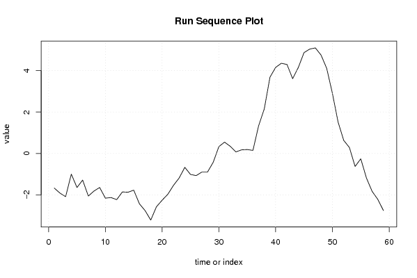
Title produced by software

Univariate Explorative Data Analysis

Date of computation

Sat, 07 Nov 2009 09:50:34 -0700

Cite this page as follows

Statistical Computations at FreeStatistics.org, Office for Research Development and Education, URL https://freestatistics.org/blog/index.php?v=date/2009/Nov/07/t12576126999l3x211qjp2h312.htm/, Retrieved Mon, 06 May 2024 11:08:05 +0000

Statistical Computations at FreeStatistics.org, Office for Research Development and Education, URL https://freestatistics.org/blog/index.php?pk=54458, Retrieved Mon, 06 May 2024 11:08:05 +0000

QR Codes:

Paste this QR Code to cite your computation.

Original text written by user:

IsPrivate?

No (this computation is public)

User-defined keywords

Estimated Impact

163

Family? (F = Feedback message, R = changed R code, M = changed R Module, P = changed Parameters, D = changed Data)

-     [Univariate Data Series] [] [2009-10-12 17:11:03] [0750c128064677e728c9436fc3f45ae7]
- RMPD  [Bivariate Explorative Data Analysis] [] [2009-10-27 16:20:04] [aa744e95cb7911d3facfcbb134d2ed3f]
-  M D    [Bivariate Explorative Data Analysis] [] [2009-11-03 14:04:11] [0750c128064677e728c9436fc3f45ae7]
- RMPD      [Univariate Summary Statistics] [] [2009-11-04 14:54:00] [0750c128064677e728c9436fc3f45ae7]
- RMPD          [Univariate Explorative Data Analysis] [Run Sequence plot...] [2009-11-07 16:50:34] [852eae237d08746109043531619a60c9] [Current]

Feedback Forum

Post a new message

Dataseries X:

Download CSV

Histogram

Boxplots

-1.666073923
-1.908115119
-2.079135718
-0.995053325
-1.637094521
-1.280563624
-2.050156316
-1.808115119
-1.637094521
-2.151584222
-2.12260482
-2.22260482
-1.851584222
-1.866073923
-1.766073923
-2.42260482
-2.751584222
-3.208115119
-2.566073923
-2.251584222
-1.966073923
-1.537094521
-1.180563624
-0.666073923
-1.008115119
-1.064646017
-0.893625419
-0.893625419
-0.42260482
0.333926077
0.548415778
0.348415778
0.07739518
0.17739518
0.191884881
0.149843684
1.335353983
2.149843684
3.67739518
4.149843684
4.349843684
4.291884881
3.607802488
4.149843684
4.862905479
5.033926077
5.090456974
4.746987872
4.103518769
2.903518769
1.51800847
0.632498171
0.289029068
-0.624032727
-0.254440035
-1.18199153
-1.824032727
-2.209543026
-2.751584222

Summary of computational transaction
Raw Input	view raw input (R code)
Raw Output	view raw output of R engine
Computing time	4 seconds
R Server	'Sir Ronald Aylmer Fisher' @ 193.190.124.24

\begin{tabular}{lllllllll}
\hline
Summary of computational transaction \tabularnewline
Raw Input & view raw input (R code)  \tabularnewline
Raw Output & view raw output of R engine  \tabularnewline
Computing time & 4 seconds \tabularnewline
R Server & 'Sir Ronald Aylmer Fisher' @ 193.190.124.24 \tabularnewline
\hline
\end{tabular}
%Source: https://freestatistics.org/blog/index.php?pk=54458&T=0

[TABLE]
[ROW][C]Summary of computational transaction[/C][/ROW]
[ROW][C]Raw Input[/C][C]view raw input (R code) [/C][/ROW]
[ROW][C]Raw Output[/C][C]view raw output of R engine [/C][/ROW]
[ROW][C]Computing time[/C][C]4 seconds[/C][/ROW]
[ROW][C]R Server[/C][C]'Sir Ronald Aylmer Fisher' @ 193.190.124.24[/C][/ROW]
[/TABLE]
Source: https://freestatistics.org/blog/index.php?pk=54458&T=0

Globally Unique Identifier (entire table): ba.freestatistics.org/blog/index.php?pk=54458&T=0

As an alternative you can also use a QR Code:

The GUIDs for individual cells are displayed in the table below:

Summary of computational transaction
Raw Input	view raw input (R code)
Raw Output	view raw output of R engine
Computing time	4 seconds
R Server	'Sir Ronald Aylmer Fisher' @ 193.190.124.24

Descriptive Statistics
# observations	59
minimum	-3.208115119
Q1	-1.8588290725
median	-0.893625419
mean	1.69491806198008e-11
Q3	0.983926077
maximum	5.090456974

\begin{tabular}{lllllllll}
\hline
Descriptive Statistics \tabularnewline
# observations & 59 \tabularnewline
minimum & -3.208115119 \tabularnewline
Q1 & -1.8588290725 \tabularnewline
median & -0.893625419 \tabularnewline
mean & 1.69491806198008e-11 \tabularnewline
Q3 & 0.983926077 \tabularnewline
maximum & 5.090456974 \tabularnewline
\hline
\end{tabular}
%Source: https://freestatistics.org/blog/index.php?pk=54458&T=1

[TABLE]
[ROW][C]Descriptive Statistics[/C][/ROW]
[ROW][C]# observations[/C][C]59[/C][/ROW]
[ROW][C]minimum[/C][C]-3.208115119[/C][/ROW]
[ROW][C]Q1[/C][C]-1.8588290725[/C][/ROW]
[ROW][C]median[/C][C]-0.893625419[/C][/ROW]
[ROW][C]mean[/C][C]1.69491806198008e-11[/C][/ROW]
[ROW][C]Q3[/C][C]0.983926077[/C][/ROW]
[ROW][C]maximum[/C][C]5.090456974[/C][/ROW]
[/TABLE]
Source: https://freestatistics.org/blog/index.php?pk=54458&T=1

Globally Unique Identifier (entire table): ba.freestatistics.org/blog/index.php?pk=54458&T=1

As an alternative you can also use a QR Code:

The GUIDs for individual cells are displayed in the table below:

Descriptive Statistics
# observations	59
minimum	-3.208115119
Q1	-1.8588290725
median	-0.893625419
mean	1.69491806198008e-11
Q3	0.983926077
maximum	5.090456974

Figure 1

PNG link

Postscript link

PDF link

Figure 2

PNG link

Postscript link

PDF link

Figure 3

PNG link

Postscript link

PDF link

Figure 4

PNG link

Postscript link

PDF link

Figure 5

PNG link

Postscript link

PDF link

Figure 6

PNG link

Postscript link

PDF link

Figure 7

PNG link

Postscript link

PDF link

Parameters (Session):

par1 = 0 ; par2 = 36 ;

Parameters (R input):

par1 = 0 ; par2 = 36 ;

R code (references can be found in the software module):

par1 <- as.numeric(par1)
par2 <- as.numeric(par2)
x <- as.ts(x)
library(lattice)
bitmap(file='pic1.png')
plot(x,type='l',main='Run Sequence Plot',xlab='time or index',ylab='value')
grid()
dev.off()
bitmap(file='pic2.png')
hist(x)
grid()
dev.off()
bitmap(file='pic3.png')
if (par1 > 0)
{
densityplot(~x,col='black',main=paste('Density Plot   bw = ',par1),bw=par1)
} else {
densityplot(~x,col='black',main='Density Plot')
}
dev.off()
bitmap(file='pic4.png')
qqnorm(x)
qqline(x)
grid()
dev.off()
if (par2 > 0)
{
bitmap(file='lagplot1.png')
dum <- cbind(lag(x,k=1),x)
dum
dum1 <- dum[2:length(x),]
dum1
z <- as.data.frame(dum1)
z
plot(z,main='Lag plot (k=1), lowess, and regression line')
lines(lowess(z))
abline(lm(z))
dev.off()
if (par2 > 1) {
bitmap(file='lagplotpar2.png')
dum <- cbind(lag(x,k=par2),x)
dum
dum1 <- dum[(par2+1):length(x),]
dum1
z <- as.data.frame(dum1)
z
mylagtitle <- 'Lag plot (k='
mylagtitle <- paste(mylagtitle,par2,sep='')
mylagtitle <- paste(mylagtitle,'), and lowess',sep='')
plot(z,main=mylagtitle)
lines(lowess(z))
dev.off()
}
bitmap(file='pic5.png')
acf(x,lag.max=par2,main='Autocorrelation Function')
grid()
dev.off()
}
summary(x)
load(file='createtable')
a<-table.start()
a<-table.row.start(a)
a<-table.element(a,'Descriptive Statistics',2,TRUE)
a<-table.row.end(a)
a<-table.row.start(a)
a<-table.element(a,'# observations',header=TRUE)
a<-table.element(a,length(x))
a<-table.row.end(a)
a<-table.row.start(a)
a<-table.element(a,'minimum',header=TRUE)
a<-table.element(a,min(x))
a<-table.row.end(a)
a<-table.row.start(a)
a<-table.element(a,'Q1',header=TRUE)
a<-table.element(a,quantile(x,0.25))
a<-table.row.end(a)
a<-table.row.start(a)
a<-table.element(a,'median',header=TRUE)
a<-table.element(a,median(x))
a<-table.row.end(a)
a<-table.row.start(a)
a<-table.element(a,'mean',header=TRUE)
a<-table.element(a,mean(x))
a<-table.row.end(a)
a<-table.row.start(a)
a<-table.element(a,'Q3',header=TRUE)
a<-table.element(a,quantile(x,0.75))
a<-table.row.end(a)
a<-table.row.start(a)
a<-table.element(a,'maximum',header=TRUE)
a<-table.element(a,max(x))
a<-table.row.end(a)
a<-table.end(a)
table.save(a,file='mytable.tab')

Free Statistics

Description of Statistical Computation

Tree of Dependent Computations

Dataset

Tables (Output of Computation)

Figures (Output of Computation)

Input Parameters & R Code