Free Statistics
of Irreproducible Research!
Description of Statistical Computation | |||||||||||||||||||||||||||||||||||||||||||||||||
|---|---|---|---|---|---|---|---|---|---|---|---|---|---|---|---|---|---|---|---|---|---|---|---|---|---|---|---|---|---|---|---|---|---|---|---|---|---|---|---|---|---|---|---|---|---|---|---|---|---|
| Author's title | |||||||||||||||||||||||||||||||||||||||||||||||||
| Author | *The author of this computation has been verified* | ||||||||||||||||||||||||||||||||||||||||||||||||
| R Software Module | rwasp_tukeylambda.wasp | ||||||||||||||||||||||||||||||||||||||||||||||||
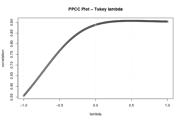
| Title produced by software | Tukey lambda PPCC Plot | ||||||||||||||||||||||||||||||||||||||||||||||||
| Date of computation | Thu, 05 Nov 2009 07:10:05 -0700 | ||||||||||||||||||||||||||||||||||||||||||||||||
| Cite this page as follows | Statistical Computations at FreeStatistics.org, Office for Research Development and Education, URL https://freestatistics.org/blog/index.php?v=date/2009/Nov/05/t1257430454st50yxfcsx277hm.htm/, Retrieved Wed, 09 Jul 2025 18:53:39 +0000 | ||||||||||||||||||||||||||||||||||||||||||||||||
| Statistical Computations at FreeStatistics.org, Office for Research Development and Education, URL https://freestatistics.org/blog/index.php?pk=54119, Retrieved Wed, 09 Jul 2025 18:53:39 +0000 | |||||||||||||||||||||||||||||||||||||||||||||||||
| QR Codes: | |||||||||||||||||||||||||||||||||||||||||||||||||
|
| |||||||||||||||||||||||||||||||||||||||||||||||||
| Original text written by user: | |||||||||||||||||||||||||||||||||||||||||||||||||
| IsPrivate? | No (this computation is public) | ||||||||||||||||||||||||||||||||||||||||||||||||
| User-defined keywords | |||||||||||||||||||||||||||||||||||||||||||||||||
| Estimated Impact | 240 | ||||||||||||||||||||||||||||||||||||||||||||||||
Tree of Dependent Computations | |||||||||||||||||||||||||||||||||||||||||||||||||
| Family? (F = Feedback message, R = changed R code, M = changed R Module, P = changed Parameters, D = changed Data) | |||||||||||||||||||||||||||||||||||||||||||||||||
| - [Tukey lambda PPCC Plot] [3/11/2009] [2009-11-02 22:14:51] [b98453cac15ba1066b407e146608df68] - PD [Tukey lambda PPCC Plot] [Tukey Lambda PPCC...] [2009-11-05 14:10:05] [9be6fbb216efe5bb8ca600257c6e1971] [Current] - D [Tukey lambda PPCC Plot] [Tukey Lamba BDM] [2009-11-10 12:22:51] [f5d341d4bbba73282fc6e80153a6d315] - [Tukey lambda PPCC Plot] [tg15] [2009-11-10 14:44:02] [a21bac9c8d3d56fdec8be4e719e2c7ed] - R [Tukey lambda PPCC Plot] [ws6] [2009-11-15 22:42:09] [3fc64fd7a52ce121dfe13dba27bf6e5b] - [Tukey lambda PPCC Plot] [TVD 15] [2009-11-10 22:44:21] [42ad1186d39724f834063794eac7cea3] - [Tukey lambda PPCC Plot] [PA15] [2009-12-15 10:03:02] [a21bac9c8d3d56fdec8be4e719e2c7ed] - PD [Tukey lambda PPCC Plot] [WS6 Tukey] [2009-11-13 19:37:41] [445b292c553470d9fed8bc2796fd3a00] - D [Tukey lambda PPCC Plot] [WS6 Review] [2009-11-18 18:26:38] [445b292c553470d9fed8bc2796fd3a00] | |||||||||||||||||||||||||||||||||||||||||||||||||
| Feedback Forum | |||||||||||||||||||||||||||||||||||||||||||||||||
Post a new message | |||||||||||||||||||||||||||||||||||||||||||||||||
Dataset | |||||||||||||||||||||||||||||||||||||||||||||||||
| Dataseries X: | |||||||||||||||||||||||||||||||||||||||||||||||||
89.3 90.3 91.1 90.1 86.7 85.1 83.4 82 80.4 81.9 93.8 94.8 92.3 87.5 83.2 82 80.3 81.8 85.1 84.2 84.4 84.5 93.3 93.2 100.3 111.4 114.9 109.5 109.9 105.8 110.8 108.8 116.1 109.8 113.8 113.8 117.4 119.5 122.6 120.7 119 126.1 133.9 138.1 140.4 148.2 148.2 155.9 171.1 171.9 188.8 214.9 228.5 220 225.4 220.7 219.7 232.1 223.5 218.9 | |||||||||||||||||||||||||||||||||||||||||||||||||
Tables (Output of Computation) | |||||||||||||||||||||||||||||||||||||||||||||||||
| |||||||||||||||||||||||||||||||||||||||||||||||||
Figures (Output of Computation) | |||||||||||||||||||||||||||||||||||||||||||||||||
Input Parameters & R Code | |||||||||||||||||||||||||||||||||||||||||||||||||
| Parameters (Session): | |||||||||||||||||||||||||||||||||||||||||||||||||
| par1 = 50 ; par2 = 50 ; par3 = 0 ; par4 = 0 ; par5 = 0 ; par6 = Y ; par7 = Y ; | |||||||||||||||||||||||||||||||||||||||||||||||||
| Parameters (R input): | |||||||||||||||||||||||||||||||||||||||||||||||||
| R code (references can be found in the software module): | |||||||||||||||||||||||||||||||||||||||||||||||||
gp <- function(lambda, p) | |||||||||||||||||||||||||||||||||||||||||||||||||