Free Statistics
of Irreproducible Research!
Description of Statistical Computation | |||||||||||||||||||||||||||||||||||||||||||||||||||||||||||||||||
|---|---|---|---|---|---|---|---|---|---|---|---|---|---|---|---|---|---|---|---|---|---|---|---|---|---|---|---|---|---|---|---|---|---|---|---|---|---|---|---|---|---|---|---|---|---|---|---|---|---|---|---|---|---|---|---|---|---|---|---|---|---|---|---|---|---|
| Author's title | |||||||||||||||||||||||||||||||||||||||||||||||||||||||||||||||||
| Author | *The author of this computation has been verified* | ||||||||||||||||||||||||||||||||||||||||||||||||||||||||||||||||
| R Software Module | rwasp_edabi.wasp | ||||||||||||||||||||||||||||||||||||||||||||||||||||||||||||||||
| Title produced by software | Bivariate Explorative Data Analysis | ||||||||||||||||||||||||||||||||||||||||||||||||||||||||||||||||
| Date of computation | Thu, 05 Nov 2009 01:48:18 -0700 | ||||||||||||||||||||||||||||||||||||||||||||||||||||||||||||||||
| Cite this page as follows | Statistical Computations at FreeStatistics.org, Office for Research Development and Education, URL https://freestatistics.org/blog/index.php?v=date/2009/Nov/05/t1257410950uclp9y3plsud1kl.htm/, Retrieved Fri, 03 May 2024 03:35:38 +0000 | ||||||||||||||||||||||||||||||||||||||||||||||||||||||||||||||||
| Statistical Computations at FreeStatistics.org, Office for Research Development and Education, URL https://freestatistics.org/blog/index.php?pk=53888, Retrieved Fri, 03 May 2024 03:35:38 +0000 | |||||||||||||||||||||||||||||||||||||||||||||||||||||||||||||||||
| QR Codes: | |||||||||||||||||||||||||||||||||||||||||||||||||||||||||||||||||
|
| |||||||||||||||||||||||||||||||||||||||||||||||||||||||||||||||||
| Original text written by user: | |||||||||||||||||||||||||||||||||||||||||||||||||||||||||||||||||
| IsPrivate? | No (this computation is public) | ||||||||||||||||||||||||||||||||||||||||||||||||||||||||||||||||
| User-defined keywords | |||||||||||||||||||||||||||||||||||||||||||||||||||||||||||||||||
| Estimated Impact | 156 | ||||||||||||||||||||||||||||||||||||||||||||||||||||||||||||||||
Tree of Dependent Computations | |||||||||||||||||||||||||||||||||||||||||||||||||||||||||||||||||
| Family? (F = Feedback message, R = changed R code, M = changed R Module, P = changed Parameters, D = changed Data) | |||||||||||||||||||||||||||||||||||||||||||||||||||||||||||||||||
| F [Partial Correlation] [WS5] [2009-11-04 17:31:42] [868ad9c0049635b9b2c3848f186e9622] - RMPD [Bivariate Explorative Data Analysis] [reeks X t.o.v Z] [2009-11-05 08:48:18] [ea241b681aafed79da4b5b99fad98471] [Current] - D [Bivariate Explorative Data Analysis] [reeks Y t.o.v. Z] [2009-11-05 08:51:09] [cd6314e7e707a6546bd4604c9d1f2b69] - D [Bivariate Explorative Data Analysis] [reeks e(t) t.o.v....] [2009-11-05 08:57:02] [cd6314e7e707a6546bd4604c9d1f2b69] - RMPD [Pearson Correlation] [check correlatie ...] [2009-11-05 08:59:04] [cd6314e7e707a6546bd4604c9d1f2b69] | |||||||||||||||||||||||||||||||||||||||||||||||||||||||||||||||||
| Feedback Forum | |||||||||||||||||||||||||||||||||||||||||||||||||||||||||||||||||
Post a new message | |||||||||||||||||||||||||||||||||||||||||||||||||||||||||||||||||
Dataset | |||||||||||||||||||||||||||||||||||||||||||||||||||||||||||||||||
| Dataseries X: | |||||||||||||||||||||||||||||||||||||||||||||||||||||||||||||||||
1,75 1,75 1,55 1,5 1,5 1,1 1 1 1 1 1 1 1 1 1 1 1 1 1 1 1 1 1 1 1 1 1 1 1 1 1 1 1 1 1 1,21 1,25 1,25 1,45 1,5 1,5 1,64 1,75 1,93 2 2,17 2,25 2,39 2,5 2,5 2,65 2,75 2,75 2,9 3 3 3 3 3 3 3 3 3 3 3 3 3,18 3,25 3,25 3,23 2,92 2,25 | |||||||||||||||||||||||||||||||||||||||||||||||||||||||||||||||||
| Dataseries Y: | |||||||||||||||||||||||||||||||||||||||||||||||||||||||||||||||||
2,93 2,76 2,51 2,51 2,48 2,24 2,12 2,1 2,13 2,12 2,14 2,13 2,13 2,04 2,02 1,92 2,03 2,05 2,08 2,08 2,08 2,08 2,12 2,14 2,13 2,1 2,09 2,1 2,09 2,08 2,07 2,08 2,09 2,11 2,2 2,42 2,46 2,5 2,59 2,75 2,78 2,9 3,03 3,1 3,23 3,36 3,51 3,61 3,67 3,74 3,82 3,89 3,98 4,08 4,14 4,33 4,57 4,63 4,57 4,71 4,54 4,3 4,36 4,61 4,71 4,68 4,91 4,75 4,77 5,18 3,42 2,71 | |||||||||||||||||||||||||||||||||||||||||||||||||||||||||||||||||
Tables (Output of Computation) | |||||||||||||||||||||||||||||||||||||||||||||||||||||||||||||||||
| |||||||||||||||||||||||||||||||||||||||||||||||||||||||||||||||||
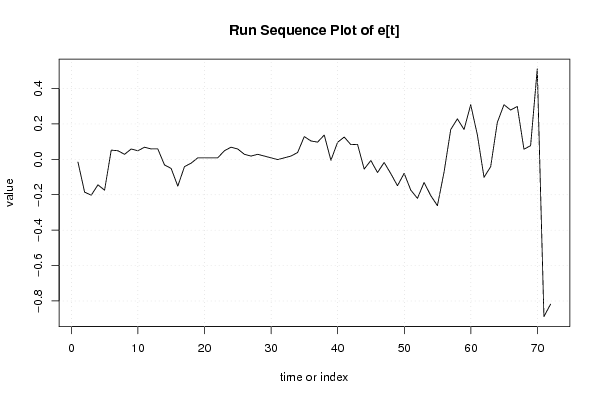
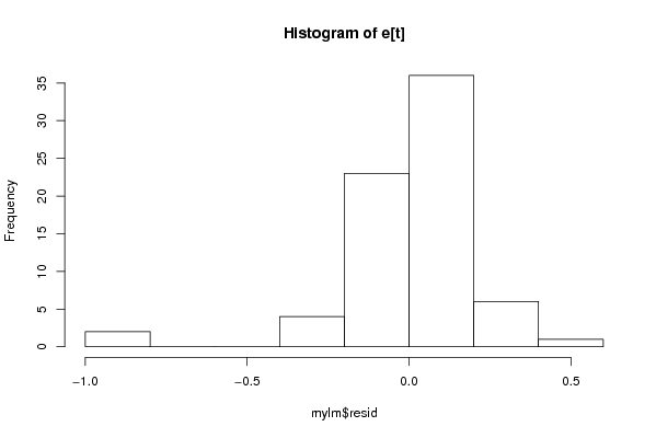
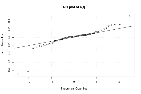
Figures (Output of Computation) | |||||||||||||||||||||||||||||||||||||||||||||||||||||||||||||||||
Input Parameters & R Code | |||||||||||||||||||||||||||||||||||||||||||||||||||||||||||||||||
| Parameters (Session): | |||||||||||||||||||||||||||||||||||||||||||||||||||||||||||||||||
| par1 = 0 ; par2 = 36 ; | |||||||||||||||||||||||||||||||||||||||||||||||||||||||||||||||||
| Parameters (R input): | |||||||||||||||||||||||||||||||||||||||||||||||||||||||||||||||||
| par1 = 0 ; par2 = 36 ; | |||||||||||||||||||||||||||||||||||||||||||||||||||||||||||||||||
| R code (references can be found in the software module): | |||||||||||||||||||||||||||||||||||||||||||||||||||||||||||||||||
par1 <- as.numeric(par1) | |||||||||||||||||||||||||||||||||||||||||||||||||||||||||||||||||