Repository of Reproducible Computations

Free Statistics

of Irreproducible Research!

Author's title

Author

*The author of this computation has been verified*

R Software Module

rwasp_edabi.wasp

Title produced by software

Bivariate Explorative Data Analysis

Date of computation

Mon, 02 Nov 2009 08:10:26 -0700

Cite this page as follows

Statistical Computations at FreeStatistics.org, Office for Research Development and Education, URL https://freestatistics.org/blog/index.php?v=date/2009/Nov/02/t12571747352jjle4ch3w5ohki.htm/, Retrieved Fri, 03 May 2024 23:29:49 +0000

Statistical Computations at FreeStatistics.org, Office for Research Development and Education, URL https://freestatistics.org/blog/index.php?pk=52702, Retrieved Fri, 03 May 2024 23:29:49 +0000

QR Codes:

Paste this QR Code to cite your computation.

Original text written by user:

IsPrivate?

No (this computation is public)

User-defined keywords

Estimated Impact

157

Family? (F = Feedback message, R = changed R code, M = changed R Module, P = changed Parameters, D = changed Data)

-     [Univariate Data Series] [Rente] [2009-10-11 21:57:47] [badc6a9acdc45286bea7f74742e15a21]
-   PD  [Univariate Data Series] [Industri�le produ...] [2009-10-12 20:03:03] [badc6a9acdc45286bea7f74742e15a21]
- RMPD    [Trivariate Scatterplots] [] [2009-11-02 13:17:40] [badc6a9acdc45286bea7f74742e15a21]
- RMPD      [Bivariate Explorative Data Analysis] [] [2009-11-02 14:03:49] [badc6a9acdc45286bea7f74742e15a21]
-    D          [Bivariate Explorative Data Analysis] [] [2009-11-02 15:10:26] [0545e25c765ce26b196961216dc11e13] [Current]
-    D            [Bivariate Explorative Data Analysis] [] [2009-11-02 15:22:24] [badc6a9acdc45286bea7f74742e15a21] 
-                 [Bivariate Explorative Data Analysis] [] [2009-11-02 16:40:48] [2c5be225250d91402426bbbf07a5e2b3] 
-    D            [Bivariate Explorative Data Analysis] [] [2009-11-02 16:43:33] [2c5be225250d91402426bbbf07a5e2b3] 

Feedback Forum

Post a new message

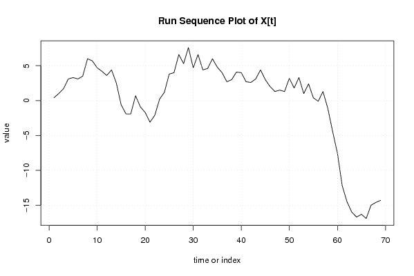
Dataseries X:

Download CSV

Histogram

Boxplots

0,4
1
1,7
3,1
3,3
3,1
3,5
6
5,7
4,7
4,2
3,6
4,4
2,5
-0,6
-1,9
-1,9
0,7
-0,9
-1,7
-3,1
-2,1
0,2
1,2
3,8
4
6,6
5,3
7,6
4,7
6,6
4,4
4,6
6
4,8
4
2,7
3
4,1
4
2,7
2,6
3,1
4,4
3
2
1,3
1,5
1,3
3,2
1,8
3,3
1
2,4
0,4
-0,1
1,3
-1,1
-4,4
-7,5
-12,2
-14,5
-16
-16,7
-16,3
-16,9
-15
-14,6
-14,3

Dataseries Y:

Download CSV

Histogram

1,4
1,2
1
1,7
2,4
2
2,1
2
1,8
2,7
2,3
1,9
2
2,3
2,8
2,4
2,3
2,7
2,7
2,9
3
2,2
2,3
2,8
2,8
2,8
2,2
2,6
2,8
2,5
2,4
2,3
1,9
1,7
2
2,1
1,7
1,8
1,8
1,8
1,3
1,3
1,3
1,2
1,4
2,2
2,9
3,1
3,5
3,6
4,4
4,1
5,1
5,8
5,9
5,4
5,5
4,8
3,2
2,7
2,1
1,9
0,6
0,7
-0,2
-1
-1,7
-0,7
-1

Summary of computational transaction
Raw Input	view raw input (R code)
Raw Output	view raw output of R engine
Computing time	4 seconds
R Server	'Gwilym Jenkins' @ 72.249.127.135

\begin{tabular}{lllllllll}
\hline
Summary of computational transaction \tabularnewline
Raw Input & view raw input (R code)  \tabularnewline
Raw Output & view raw output of R engine  \tabularnewline
Computing time & 4 seconds \tabularnewline
R Server & 'Gwilym Jenkins' @ 72.249.127.135 \tabularnewline
\hline
\end{tabular}
%Source: https://freestatistics.org/blog/index.php?pk=52702&T=0

[TABLE]
[ROW][C]Summary of computational transaction[/C][/ROW]
[ROW][C]Raw Input[/C][C]view raw input (R code) [/C][/ROW]
[ROW][C]Raw Output[/C][C]view raw output of R engine [/C][/ROW]
[ROW][C]Computing time[/C][C]4 seconds[/C][/ROW]
[ROW][C]R Server[/C][C]'Gwilym Jenkins' @ 72.249.127.135[/C][/ROW]
[/TABLE]
Source: https://freestatistics.org/blog/index.php?pk=52702&T=0

Globally Unique Identifier (entire table): ba.freestatistics.org/blog/index.php?pk=52702&T=0

As an alternative you can also use a QR Code:

The GUIDs for individual cells are displayed in the table below:

Summary of computational transaction
Raw Input	view raw input (R code)
Raw Output	view raw output of R engine
Computing time	4 seconds
R Server	'Gwilym Jenkins' @ 72.249.127.135

Model: Y[t] = c + b X[t] + e[t]
c	2.28411241749877
b	0.103756807415105

\begin{tabular}{lllllllll}
\hline
Model: Y[t] = c + b X[t] + e[t] \tabularnewline
c & 2.28411241749877 \tabularnewline
b & 0.103756807415105 \tabularnewline
\hline
\end{tabular}
%Source: https://freestatistics.org/blog/index.php?pk=52702&T=1

[TABLE]
[ROW][C]Model: Y[t] = c + b X[t] + e[t][/C][/ROW]
[ROW][C]c[/C][C]2.28411241749877[/C][/ROW]
[ROW][C]b[/C][C]0.103756807415105[/C][/ROW]
[/TABLE]
Source: https://freestatistics.org/blog/index.php?pk=52702&T=1

Globally Unique Identifier (entire table): ba.freestatistics.org/blog/index.php?pk=52702&T=1

As an alternative you can also use a QR Code:

The GUIDs for individual cells are displayed in the table below:

Model: Y[t] = c + b X[t] + e[t]
c	2.28411241749877
b	0.103756807415105

Descriptive Statistics about e[t]
# observations	69
minimum	-2.4277603062722
Q1	-0.899139647159188
median	-0.271769412349762
mean	6.97440545332487e-17
Q3	0.578141666950293
maximum	3.57438485953519

\begin{tabular}{lllllllll}
\hline
Descriptive Statistics about e[t] \tabularnewline
# observations & 69 \tabularnewline
minimum & -2.4277603062722 \tabularnewline
Q1 & -0.899139647159188 \tabularnewline
median & -0.271769412349762 \tabularnewline
mean & 6.97440545332487e-17 \tabularnewline
Q3 & 0.578141666950293 \tabularnewline
maximum & 3.57438485953519 \tabularnewline
\hline
\end{tabular}
%Source: https://freestatistics.org/blog/index.php?pk=52702&T=2

[TABLE]
[ROW][C]Descriptive Statistics about e[t][/C][/ROW]
[ROW][C]# observations[/C][C]69[/C][/ROW]
[ROW][C]minimum[/C][C]-2.4277603062722[/C][/ROW]
[ROW][C]Q1[/C][C]-0.899139647159188[/C][/ROW]
[ROW][C]median[/C][C]-0.271769412349762[/C][/ROW]
[ROW][C]mean[/C][C]6.97440545332487e-17[/C][/ROW]
[ROW][C]Q3[/C][C]0.578141666950293[/C][/ROW]
[ROW][C]maximum[/C][C]3.57438485953519[/C][/ROW]
[/TABLE]
Source: https://freestatistics.org/blog/index.php?pk=52702&T=2

Globally Unique Identifier (entire table): ba.freestatistics.org/blog/index.php?pk=52702&T=2

As an alternative you can also use a QR Code:

The GUIDs for individual cells are displayed in the table below:

Descriptive Statistics about e[t]
# observations	69
minimum	-2.4277603062722
Q1	-0.899139647159188
median	-0.271769412349762
mean	6.97440545332487e-17
Q3	0.578141666950293
maximum	3.57438485953519

Figure 1

PNG link

Postscript link

PDF link

Figure 2

PNG link

Postscript link

PDF link

Figure 3

PNG link

Postscript link

PDF link

Figure 4

PNG link

Postscript link

PDF link

Figure 5

PNG link

Postscript link

PDF link

Figure 6

PNG link

Postscript link

PDF link

Figure 7

PNG link

Postscript link

PDF link

Figure 8

PNG link

Postscript link

PDF link

Parameters (Session):

par1 = 0 ; par2 = 36 ;

Parameters (R input):

par1 = 0 ; par2 = 36 ;

R code (references can be found in the software module):

par1 <- as.numeric(par1)
par2 <- as.numeric(par2)
x <- as.ts(x)
y <- as.ts(y)
mylm <- lm(y~x)
cbind(mylm$resid)
library(lattice)
bitmap(file='pic1.png')
plot(y,type='l',main='Run Sequence Plot of Y[t]',xlab='time or index',ylab='value')
grid()
dev.off()
bitmap(file='pic1a.png')
plot(x,type='l',main='Run Sequence Plot of X[t]',xlab='time or index',ylab='value')
grid()
dev.off()
bitmap(file='pic1b.png')
plot(x,y,main='Scatter Plot',xlab='X[t]',ylab='Y[t]')
grid()
dev.off()
bitmap(file='pic1c.png')
plot(mylm$resid,type='l',main='Run Sequence Plot of e[t]',xlab='time or index',ylab='value')
grid()
dev.off()
bitmap(file='pic2.png')
hist(mylm$resid,main='Histogram of e[t]')
dev.off()
bitmap(file='pic3.png')
if (par1 > 0)
{
densityplot(~mylm$resid,col='black',main=paste('Density Plot of e[t]   bw = ',par1),bw=par1)
} else {
densityplot(~mylm$resid,col='black',main='Density Plot of e[t]')
}
dev.off()
bitmap(file='pic4.png')
qqnorm(mylm$resid,main='QQ plot of e[t]')
qqline(mylm$resid)
grid()
dev.off()
if (par2 > 0)
{
bitmap(file='pic5.png')
acf(mylm$resid,lag.max=par2,main='Residual Autocorrelation Function')
grid()
dev.off()
}
summary(x)
load(file='createtable')
a<-table.start()
a<-table.row.start(a)
a<-table.element(a,'Model: Y[t] = c + b X[t] + e[t]',2,TRUE)
a<-table.row.end(a)
a<-table.row.start(a)
a<-table.element(a,'c',1,TRUE)
a<-table.element(a,mylm$coeff[[1]])
a<-table.row.end(a)
a<-table.row.start(a)
a<-table.element(a,'b',1,TRUE)
a<-table.element(a,mylm$coeff[[2]])
a<-table.row.end(a)
a<-table.end(a)
table.save(a,file='mytable.tab')
a<-table.start()
a<-table.row.start(a)
a<-table.element(a,'Descriptive Statistics about e[t]',2,TRUE)
a<-table.row.end(a)
a<-table.row.start(a)
a<-table.element(a,'# observations',header=TRUE)
a<-table.element(a,length(mylm$resid))
a<-table.row.end(a)
a<-table.row.start(a)
a<-table.element(a,'minimum',header=TRUE)
a<-table.element(a,min(mylm$resid))
a<-table.row.end(a)
a<-table.row.start(a)
a<-table.element(a,'Q1',header=TRUE)
a<-table.element(a,quantile(mylm$resid,0.25))
a<-table.row.end(a)
a<-table.row.start(a)
a<-table.element(a,'median',header=TRUE)
a<-table.element(a,median(mylm$resid))
a<-table.row.end(a)
a<-table.row.start(a)
a<-table.element(a,'mean',header=TRUE)
a<-table.element(a,mean(mylm$resid))
a<-table.row.end(a)
a<-table.row.start(a)
a<-table.element(a,'Q3',header=TRUE)
a<-table.element(a,quantile(mylm$resid,0.75))
a<-table.row.end(a)
a<-table.row.start(a)
a<-table.element(a,'maximum',header=TRUE)
a<-table.element(a,max(mylm$resid))
a<-table.row.end(a)
a<-table.end(a)
table.save(a,file='mytable.tab')

Free Statistics

Description of Statistical Computation

Tree of Dependent Computations

Dataset

Tables (Output of Computation)

Figures (Output of Computation)

Input Parameters & R Code