Free Statistics
of Irreproducible Research!
Description of Statistical Computation | |||||||||||||||||||||||||||||||||||||||||||||||||||||||||||||||||
|---|---|---|---|---|---|---|---|---|---|---|---|---|---|---|---|---|---|---|---|---|---|---|---|---|---|---|---|---|---|---|---|---|---|---|---|---|---|---|---|---|---|---|---|---|---|---|---|---|---|---|---|---|---|---|---|---|---|---|---|---|---|---|---|---|---|
| Author's title | |||||||||||||||||||||||||||||||||||||||||||||||||||||||||||||||||
| Author | *The author of this computation has been verified* | ||||||||||||||||||||||||||||||||||||||||||||||||||||||||||||||||
| R Software Module | rwasp_edabi.wasp | ||||||||||||||||||||||||||||||||||||||||||||||||||||||||||||||||
| Title produced by software | Bivariate Explorative Data Analysis | ||||||||||||||||||||||||||||||||||||||||||||||||||||||||||||||||
| Date of computation | Mon, 02 Nov 2009 07:48:25 -0700 | ||||||||||||||||||||||||||||||||||||||||||||||||||||||||||||||||
| Cite this page as follows | Statistical Computations at FreeStatistics.org, Office for Research Development and Education, URL https://freestatistics.org/blog/index.php?v=date/2009/Nov/02/t1257173374a8m07s4d1ecy13k.htm/, Retrieved Fri, 03 May 2024 17:43:48 +0000 | ||||||||||||||||||||||||||||||||||||||||||||||||||||||||||||||||
| Statistical Computations at FreeStatistics.org, Office for Research Development and Education, URL https://freestatistics.org/blog/index.php?pk=52687, Retrieved Fri, 03 May 2024 17:43:48 +0000 | |||||||||||||||||||||||||||||||||||||||||||||||||||||||||||||||||
| QR Codes: | |||||||||||||||||||||||||||||||||||||||||||||||||||||||||||||||||
|
| |||||||||||||||||||||||||||||||||||||||||||||||||||||||||||||||||
| Original text written by user: | |||||||||||||||||||||||||||||||||||||||||||||||||||||||||||||||||
| IsPrivate? | No (this computation is public) | ||||||||||||||||||||||||||||||||||||||||||||||||||||||||||||||||
| User-defined keywords | |||||||||||||||||||||||||||||||||||||||||||||||||||||||||||||||||
| Estimated Impact | 150 | ||||||||||||||||||||||||||||||||||||||||||||||||||||||||||||||||
Tree of Dependent Computations | |||||||||||||||||||||||||||||||||||||||||||||||||||||||||||||||||
| Family? (F = Feedback message, R = changed R code, M = changed R Module, P = changed Parameters, D = changed Data) | |||||||||||||||||||||||||||||||||||||||||||||||||||||||||||||||||
| - [Bivariate Data Series] [Bivariate dataset] [2008-01-05 23:51:08] [74be16979710d4c4e7c6647856088456] - PD [Bivariate Data Series] [Reproduction Part 1] [2009-10-26 18:51:43] [96e597a9107bfe8c07649cce3d4f6fec] - RMPD [Bivariate Explorative Data Analysis] [JJ Workshop 4, De...] [2009-10-26 19:42:48] [96e597a9107bfe8c07649cce3d4f6fec] - D [Bivariate Explorative Data Analysis] [JJ Workshop 4, de...] [2009-10-27 18:56:34] [96e597a9107bfe8c07649cce3d4f6fec] - RM D [Bivariate Explorative Data Analysis] [JJ Workshop 5, mo...] [2009-11-02 13:36:21] [96e597a9107bfe8c07649cce3d4f6fec] - D [Bivariate Explorative Data Analysis] [JJ Workshop 5, mo...] [2009-11-02 14:48:25] [e31f2fa83f4a5291b9a51009566cf69b] [Current] | |||||||||||||||||||||||||||||||||||||||||||||||||||||||||||||||||
| Feedback Forum | |||||||||||||||||||||||||||||||||||||||||||||||||||||||||||||||||
Post a new message | |||||||||||||||||||||||||||||||||||||||||||||||||||||||||||||||||
Dataset | |||||||||||||||||||||||||||||||||||||||||||||||||||||||||||||||||
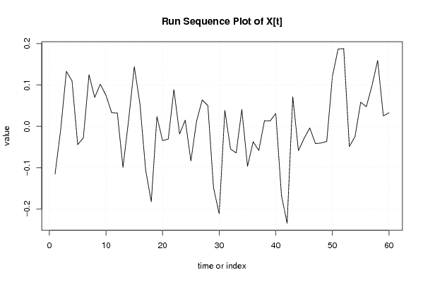
| Dataseries X: | |||||||||||||||||||||||||||||||||||||||||||||||||||||||||||||||||
-0,115348744 -0,007430684 0,133083506 0,10990307 -0,044227883 -0,027962073 0,124923169 0,069938271 0,10207697 0,074946808 0,033187327 0,032240529 -0,099390858 0,015707515 0,144498623 0,054184893 -0,105055816 -0,182509537 0,023413818 -0,034617275 -0,030773287 0,088969168 -0,018347742 0,015141613 -0,083681811 0,012257933 0,063956725 0,050285253 -0,148793116 -0,211572756 0,038835971 -0,054887315 -0,064381527 0,040560126 -0,096653186 -0,03730336 -0,058279231 0,01374282 0,012929942 0,031409519 -0,167303701 -0,234454594 0,071595677 -0,058758499 -0,029159212 -0,003939614 -0,04168033 -0,040265025 -0,036687857 0,120682129 0,186906774 0,188095521 -0,048823116 -0,02473896 0,058343008 0,047528578 0,098720517 0,159550648 0,025284856 0,032824856 | |||||||||||||||||||||||||||||||||||||||||||||||||||||||||||||||||
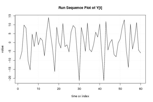
| Dataseries Y: | |||||||||||||||||||||||||||||||||||||||||||||||||||||||||||||||||
-9.314 -5.0234 9.814 8.1308 -10.2608 -15.3104 4.6961 -2.2175 6.0038 -1.2903 2.5262 1.1646 -7.4196 5.355 14.0077 4.5124 -3.8231 -16.2402 8.6444 0.0841 -3.0662 10.6491 -2.219 -1.2421 -5.2066 5.9774 9.549 8.2253 -6.2735 -21.3735 8.4939 3.0555 -4.8665 10.9275 -3.7873 -5.1465 -1.1365 5.8179 3.1025 10.4451 -6.8916 -21.2798 11.7841 -4.1934 -0.0117 1.7321 -6.8123 -7.9135 -0.168 2.0539 8.7166 12.7296 -4.5136 -13.8994 10.342 -3.6225 1.558 11.2231 -4.3136 -5.8018 | |||||||||||||||||||||||||||||||||||||||||||||||||||||||||||||||||
Tables (Output of Computation) | |||||||||||||||||||||||||||||||||||||||||||||||||||||||||||||||||
| |||||||||||||||||||||||||||||||||||||||||||||||||||||||||||||||||
Figures (Output of Computation) | |||||||||||||||||||||||||||||||||||||||||||||||||||||||||||||||||
Input Parameters & R Code | |||||||||||||||||||||||||||||||||||||||||||||||||||||||||||||||||
| Parameters (Session): | |||||||||||||||||||||||||||||||||||||||||||||||||||||||||||||||||
| par1 = 0 ; par2 = 36 ; | |||||||||||||||||||||||||||||||||||||||||||||||||||||||||||||||||
| Parameters (R input): | |||||||||||||||||||||||||||||||||||||||||||||||||||||||||||||||||
| par1 = 0 ; par2 = 36 ; | |||||||||||||||||||||||||||||||||||||||||||||||||||||||||||||||||
| R code (references can be found in the software module): | |||||||||||||||||||||||||||||||||||||||||||||||||||||||||||||||||
par1 <- as.numeric(par1) | |||||||||||||||||||||||||||||||||||||||||||||||||||||||||||||||||