Free Statistics
of Irreproducible Research!
Description of Statistical Computation | |||||||||||||||||||||
|---|---|---|---|---|---|---|---|---|---|---|---|---|---|---|---|---|---|---|---|---|---|
| Author's title | |||||||||||||||||||||
| Author | *The author of this computation has been verified* | ||||||||||||||||||||
| R Software Module | rwasp_cloud.wasp | ||||||||||||||||||||
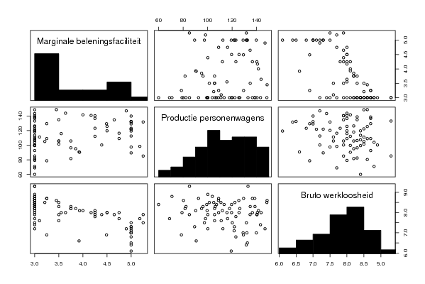
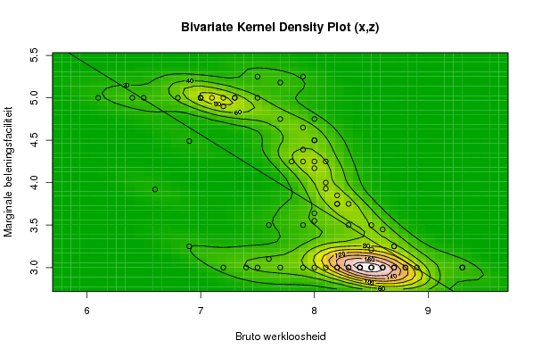
| Title produced by software | Trivariate Scatterplots | ||||||||||||||||||||
| Date of computation | Mon, 02 Nov 2009 07:03:25 -0700 | ||||||||||||||||||||
| Cite this page as follows | Statistical Computations at FreeStatistics.org, Office for Research Development and Education, URL https://freestatistics.org/blog/index.php?v=date/2009/Nov/02/t1257170713auq4r8omqr8mbaa.htm/, Retrieved Fri, 03 May 2024 23:30:08 +0000 | ||||||||||||||||||||
| Statistical Computations at FreeStatistics.org, Office for Research Development and Education, URL https://freestatistics.org/blog/index.php?pk=52643, Retrieved Fri, 03 May 2024 23:30:08 +0000 | |||||||||||||||||||||
| QR Codes: | |||||||||||||||||||||
|
| |||||||||||||||||||||
| Original text written by user: | |||||||||||||||||||||
| IsPrivate? | No (this computation is public) | ||||||||||||||||||||
| User-defined keywords | |||||||||||||||||||||
| Estimated Impact | 131 | ||||||||||||||||||||
Tree of Dependent Computations | |||||||||||||||||||||
| Family? (F = Feedback message, R = changed R code, M = changed R Module, P = changed Parameters, D = changed Data) | |||||||||||||||||||||
| - [Univariate Data Series] [WS2] [2009-10-12 16:56:43] [4f76e114ed5e444b1133aad392380aad] - RMPD [Univariate Summary Statistics] [] [2009-10-28 19:03:12] [4f76e114ed5e444b1133aad392380aad] - RMPD [Trivariate Scatterplots] [Workshop 5, Triva...] [2009-11-02 14:03:25] [852eae237d08746109043531619a60c9] [Current] | |||||||||||||||||||||
| Feedback Forum | |||||||||||||||||||||
Post a new message | |||||||||||||||||||||
Dataset | |||||||||||||||||||||
| Dataseries X: | |||||||||||||||||||||
7,8 8 8,1 8,2 8,3 8,2 8 7,9 7,6 7,6 8,3 8,4 8,4 8,4 8,4 8,6 8,9 8,8 8,3 7,5 7,2 7,4 8,8 9,3 9,3 8,7 8,2 8,3 8,5 8,6 8,5 8,2 8,1 7,9 8,6 8,7 8,7 8,5 8,4 8,5 8,7 8,7 8,6 8,5 8,3 8 8,2 8,1 8,1 8 7,9 7,9 8 8 7,9 8 7,7 7,2 7,5 7,3 7 7 7 7,2 7,3 7,1 6,8 6,4 6,1 6,5 7,7 7,9 7,5 6,9 6,6 6,9 7,7 8 | |||||||||||||||||||||
| Dataseries Y: | |||||||||||||||||||||
123,10 136,60 112,10 95,10 96,30 105,70 115,80 105,70 105,70 111,10 82,40 60,00 107,30 99,30 113,50 108,90 100,20 103,90 138,70 120,20 100,20 143,20 70,90 85,20 133,00 136,60 117,90 106,30 122,30 125,50 148,40 126,30 99,60 140,40 80,30 92,60 138,50 110,90 119,60 105,00 109,00 129,40 148,60 101,40 134,80 143,70 81,60 90,30 141,50 140,70 140,20 100,20 125,70 119,60 134,70 109,00 116,30 146,90 97,40 89,40 132,10 139,80 129,00 112,50 121,90 121,70 123,10 131,60 119,30 132,50 98,30 85,10 131,70 129,30 90,70 78,60 68,90 79,10 | |||||||||||||||||||||
| Dataseries Z: | |||||||||||||||||||||
4.25 4.25 4.25 3.85 3.75 3.75 3.55 3.5 3.5 3.1 3 3 3 3 3 3 3 3 3 3 3 3 3 3 3 3 3 3 3 3 3 3 3 3 3 3 3 3 3 3.21 3.25 3.25 3.45 3.5 3.5 3.64 3.75 3.93 4 4.17 4.25 4.39 4.5 4.5 4.65 4.75 4.75 4.9 5 5 5 5 5 5 5 5 5 5 5 5 5.18 5.25 5.25 4.49 3.92 3.25 3 3 | |||||||||||||||||||||
Tables (Output of Computation) | |||||||||||||||||||||
| |||||||||||||||||||||
Figures (Output of Computation) | |||||||||||||||||||||
Input Parameters & R Code | |||||||||||||||||||||
| Parameters (Session): | |||||||||||||||||||||
| par1 = 50 ; par2 = 50 ; par3 = Y ; par4 = Y ; par5 = Bruto werkloosheid ; par6 = Productie personenwagens ; par7 = Marginale beleningsfaciliteit ; | |||||||||||||||||||||
| Parameters (R input): | |||||||||||||||||||||
| par1 = 50 ; par2 = 50 ; par3 = Y ; par4 = Y ; par5 = Bruto werkloosheid ; par6 = Productie personenwagens ; par7 = Marginale beleningsfaciliteit ; | |||||||||||||||||||||
| R code (references can be found in the software module): | |||||||||||||||||||||
x <- array(x,dim=c(length(x),1)) | |||||||||||||||||||||