Repository of Reproducible Computations

Free Statistics

of Irreproducible Research!

Author's title

Author

*The author of this computation has been verified*

R Software Module

rwasp_edauni.wasp

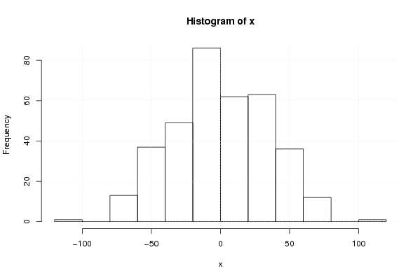
Title produced by software

Univariate Explorative Data Analysis

Date of computation

Mon, 02 Nov 2009 06:21:26 -0700

Cite this page as follows

Statistical Computations at FreeStatistics.org, Office for Research Development and Education, URL https://freestatistics.org/blog/index.php?v=date/2009/Nov/02/t1257168835qb16bo2kxx4yws0.htm/, Retrieved Fri, 03 May 2024 19:16:28 +0000

Statistical Computations at FreeStatistics.org, Office for Research Development and Education, URL https://freestatistics.org/blog/index.php?pk=52599, Retrieved Fri, 03 May 2024 19:16:28 +0000

QR Codes:

Paste this QR Code to cite your computation.

Original text written by user:

IsPrivate?

No (this computation is public)

User-defined keywords

Estimated Impact

104

Family? (F = Feedback message, R = changed R code, M = changed R Module, P = changed Parameters, D = changed Data)

-       [Univariate Explorative Data Analysis] [] [2009-11-02 13:21:26] [c4328af89eba9af53ee195d6fed304d9] [Current]

Feedback Forum

Post a new message

Dataseries X:

Download CSV

Histogram

Boxplots

-71.293676
-46.093676
-26.043753
13.569336
47.335397
60.870876
56.626127
49.84439
44.725665
39.649102
29.025203
24.811806
20.593081
17.453506
15.62702
4.326866
-0.410122
-8.383944
-13.1946
-27.486839
-34.542398
-36.898111
-36.177415
-36.277723
-39.270116
-40.386562
-30.092999
-32.303809
-36.579602
-39.043815
-20.45096
2.484057
6.322431
8.459881
10.420922
11.02123
-1.155025
6.268258
0.428529
-10.046648
-5.94711
-6.03707
2.225788
0.746484
-8.595986
-12.451699
-24.170578
-39.108921
-41.598573
-55.37529
-59.365096
-60.339072
-61.502546
-58.634514
-60.284899
-60.024782
-59.119916
-65.699959
-73.37529
-62.920347
-62.583975
-49.397526
-54.485638
-54.075136
-51.641351
-51.378647
-52.621117
-49.27683
-48.964049
-62.240581
-60.083359
-56.636639
-52.634514
-48.713972
-45.82509
-53.037563
-52.792968
-51.033005
-49.828293
-45.565743
-52.554163
-52.511847
-49.430418
-48.941536
-43.933775
-35.800144
-36.268946
-35.213695
-33.287517
-28.590412
-23.262109
-26.706242
-26.40076
-22.885546
-22.585854
-23.003963
-20.351915
-15.147357
-17.380988
-12.305965
-7.967622
-10.561678
-6.541444
-8.647388
-13.199282
-8.655303
-15.796079
-23.559245
-13.554348
52.628498
45.992342
36.595545
30.853845
29.569213
25.215933
14.570568
-1.714372
-1.241166
0.425049
3.121692
2.949995
-2.334791
-5.11699
-11.846525
-18.97606
-17.900267
-18.48764
-26.051268
-20.2359
-16.580033
-31.618838
-32.895555
-23.016559
-26.252623
-29.621733
-23.431927
-24.016405
-22.459183
-13.533467
-15.181419
-11.555703
-12.578832
-16.853393
-10.919762
-7.148681
7.23167
7.570783
3.273401
11.185874
10.07568
16.851781
14.214331
9.768966
4.450395
-9.988872
-3.586901
-2.363926
5.751134
-5.295432
-9.947172
-1.534699
5.330438
15.774571
15.837121
4.052828
6.063022
0.159819
2.503952
5.261328
9.979283
-0.004425
-3.745047
-6.108675
-5.272303
-9.328016
-15.273227
-15.710677
-17.570486
-19.747049
-22.20809
-17.90809
-8.983298
-11.257736
-11.942214
-5.945109
-8.229587
1.468873
3.738568
-2.83008
-6.298728
-15.40421
-17.072858
-17.352008
-6.467992
-4.602393
-7.90923
-4.816991
-1.627801
0.793049
-15.628078
-15.315143
-22.102208
-19.786532
-13.631589
-7.76599
-20.481635
-58.07104
-55.816251
-52.369223
-47.837255
28.820121
106.622801
78.270661
72.663824
76.361083
73.875219
79.103368
64.360898
55.591634
54.62816
47.347809
52.772755
53.182487
62.323109
59.530408
52.415933
47.094929
41.060682
35.181809
31.693389
28.522154
31.636752
21.955477
23.491849
12.719259
-15.361184
-24.615665
-28.175166
-34.348834
-17.657242
-9.498665
-42.872548
-104.104761
-47.579846
-71.219913
-39.430415
52.837893
69.258866
72.972694
61.025635
61.278884
33.505555
20.310729
2.181995
35.917997
25.423941
38.485074
32.176543
28.85326
24.418551
31.525665
22.846053
10.745622
5.156586
6.30346
10.962807
13.608018
15.333734
21.235705
13.725203
24.620152
30.116487
34.351627
43.306878
12.52625
-8.997741
27.337984
50.412237
44.004784
46.784673
43.602628
43.529391
45.618735
52.767118
43.814146
39.514608
29.701981
29.401365
36.58689
47.563268
45.976511
32.383071
22.082024
47.614546
42.432809
36.190955
32.433425
42.225787
34.019104
28.231885
26.609064
30.316363
12.094774
18.140755
32.580453
30.050456
46.676603
45.265331
34.4649
29.5649
24.376788
33.108109
41.436135
36.477681
43.307955
46.019535
36.138568
41.855599
35.825633
38.921814
37.856215
30.684672
24.556061
31.411928
21.361882
17.246206
20.426126
21.764777
11.154891
-6.927123
21.398408
19.593542
6.669982
5.387937
-15.93242
-33.867991
-7.9861
-44.080556
-62.872271
-26.051606
-11.84751
9.468135
19.335212
34.245714
39.512206
21.518797
-0.805995
-6.734914
-35.231341
-23.700944
0.141341
-2.913448
9.177251
2.950734
0.267026
-6.822595
-2.289888
-3.174674
-23.60658
-42.435006

Summary of computational transaction
Raw Input	view raw input (R code)
Raw Output	view raw output of R engine
Computing time	4 seconds
R Server	'Sir Ronald Aylmer Fisher' @ 193.190.124.24

\begin{tabular}{lllllllll}
\hline
Summary of computational transaction \tabularnewline
Raw Input & view raw input (R code)  \tabularnewline
Raw Output & view raw output of R engine  \tabularnewline
Computing time & 4 seconds \tabularnewline
R Server & 'Sir Ronald Aylmer Fisher' @ 193.190.124.24 \tabularnewline
\hline
\end{tabular}
%Source: https://freestatistics.org/blog/index.php?pk=52599&T=0

[TABLE]
[ROW][C]Summary of computational transaction[/C][/ROW]
[ROW][C]Raw Input[/C][C]view raw input (R code) [/C][/ROW]
[ROW][C]Raw Output[/C][C]view raw output of R engine [/C][/ROW]
[ROW][C]Computing time[/C][C]4 seconds[/C][/ROW]
[ROW][C]R Server[/C][C]'Sir Ronald Aylmer Fisher' @ 193.190.124.24[/C][/ROW]
[/TABLE]
Source: https://freestatistics.org/blog/index.php?pk=52599&T=0

Globally Unique Identifier (entire table): ba.freestatistics.org/blog/index.php?pk=52599&T=0

As an alternative you can also use a QR Code:

The GUIDs for individual cells are displayed in the table below:

Summary of computational transaction
Raw Input	view raw input (R code)
Raw Output	view raw output of R engine
Computing time	4 seconds
R Server	'Sir Ronald Aylmer Fisher' @ 193.190.124.24

Descriptive Statistics
# observations	360
minimum	-104.104761
Q1	-23.007112
median	-1.58125
mean	-0.00130821666666695
Q3	28.30445225
maximum	106.622801

\begin{tabular}{lllllllll}
\hline
Descriptive Statistics \tabularnewline
# observations & 360 \tabularnewline
minimum & -104.104761 \tabularnewline
Q1 & -23.007112 \tabularnewline
median & -1.58125 \tabularnewline
mean & -0.00130821666666695 \tabularnewline
Q3 & 28.30445225 \tabularnewline
maximum & 106.622801 \tabularnewline
\hline
\end{tabular}
%Source: https://freestatistics.org/blog/index.php?pk=52599&T=1

[TABLE]
[ROW][C]Descriptive Statistics[/C][/ROW]
[ROW][C]# observations[/C][C]360[/C][/ROW]
[ROW][C]minimum[/C][C]-104.104761[/C][/ROW]
[ROW][C]Q1[/C][C]-23.007112[/C][/ROW]
[ROW][C]median[/C][C]-1.58125[/C][/ROW]
[ROW][C]mean[/C][C]-0.00130821666666695[/C][/ROW]
[ROW][C]Q3[/C][C]28.30445225[/C][/ROW]
[ROW][C]maximum[/C][C]106.622801[/C][/ROW]
[/TABLE]
Source: https://freestatistics.org/blog/index.php?pk=52599&T=1

Globally Unique Identifier (entire table): ba.freestatistics.org/blog/index.php?pk=52599&T=1

As an alternative you can also use a QR Code:

The GUIDs for individual cells are displayed in the table below:

Descriptive Statistics
# observations	360
minimum	-104.104761
Q1	-23.007112
median	-1.58125
mean	-0.00130821666666695
Q3	28.30445225
maximum	106.622801

Figure 1

PNG link

Postscript link

PDF link

Figure 2

PNG link

Postscript link

PDF link

Figure 3

PNG link

Postscript link

PDF link

Figure 4

PNG link

Postscript link

PDF link

Figure 5

PNG link

Postscript link

PDF link

Figure 6

PNG link

Postscript link

PDF link

Figure 7

PNG link

Postscript link

PDF link

Parameters (Session):

par1 = 0 ; par2 = 36 ;

Parameters (R input):

par1 = 0 ; par2 = 36 ;

R code (references can be found in the software module):

par1 <- as.numeric(par1)
par2 <- as.numeric(par2)
x <- as.ts(x)
library(lattice)
bitmap(file='pic1.png')
plot(x,type='l',main='Run Sequence Plot',xlab='time or index',ylab='value')
grid()
dev.off()
bitmap(file='pic2.png')
hist(x)
grid()
dev.off()
bitmap(file='pic3.png')
if (par1 > 0)
{
densityplot(~x,col='black',main=paste('Density Plot   bw = ',par1),bw=par1)
} else {
densityplot(~x,col='black',main='Density Plot')
}
dev.off()
bitmap(file='pic4.png')
qqnorm(x)
qqline(x)
grid()
dev.off()
if (par2 > 0)
{
bitmap(file='lagplot1.png')
dum <- cbind(lag(x,k=1),x)
dum
dum1 <- dum[2:length(x),]
dum1
z <- as.data.frame(dum1)
z
plot(z,main='Lag plot (k=1), lowess, and regression line')
lines(lowess(z))
abline(lm(z))
dev.off()
if (par2 > 1) {
bitmap(file='lagplotpar2.png')
dum <- cbind(lag(x,k=par2),x)
dum
dum1 <- dum[(par2+1):length(x),]
dum1
z <- as.data.frame(dum1)
z
mylagtitle <- 'Lag plot (k='
mylagtitle <- paste(mylagtitle,par2,sep='')
mylagtitle <- paste(mylagtitle,'), and lowess',sep='')
plot(z,main=mylagtitle)
lines(lowess(z))
dev.off()
}
bitmap(file='pic5.png')
acf(x,lag.max=par2,main='Autocorrelation Function')
grid()
dev.off()
}
summary(x)
load(file='createtable')
a<-table.start()
a<-table.row.start(a)
a<-table.element(a,'Descriptive Statistics',2,TRUE)
a<-table.row.end(a)
a<-table.row.start(a)
a<-table.element(a,'# observations',header=TRUE)
a<-table.element(a,length(x))
a<-table.row.end(a)
a<-table.row.start(a)
a<-table.element(a,'minimum',header=TRUE)
a<-table.element(a,min(x))
a<-table.row.end(a)
a<-table.row.start(a)
a<-table.element(a,'Q1',header=TRUE)
a<-table.element(a,quantile(x,0.25))
a<-table.row.end(a)
a<-table.row.start(a)
a<-table.element(a,'median',header=TRUE)
a<-table.element(a,median(x))
a<-table.row.end(a)
a<-table.row.start(a)
a<-table.element(a,'mean',header=TRUE)
a<-table.element(a,mean(x))
a<-table.row.end(a)
a<-table.row.start(a)
a<-table.element(a,'Q3',header=TRUE)
a<-table.element(a,quantile(x,0.75))
a<-table.row.end(a)
a<-table.row.start(a)
a<-table.element(a,'maximum',header=TRUE)
a<-table.element(a,max(x))
a<-table.row.end(a)
a<-table.end(a)
table.save(a,file='mytable.tab')

Free Statistics

Description of Statistical Computation

Tree of Dependent Computations

Dataset

Tables (Output of Computation)

Figures (Output of Computation)

Input Parameters & R Code