Free Statistics
of Irreproducible Research!
Description of Statistical Computation | |||||||||||||||||||||
|---|---|---|---|---|---|---|---|---|---|---|---|---|---|---|---|---|---|---|---|---|---|
| Author's title | |||||||||||||||||||||
| Author | *The author of this computation has been verified* | ||||||||||||||||||||
| R Software Module | rwasp_cloud.wasp | ||||||||||||||||||||
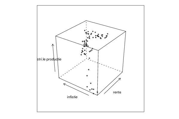
| Title produced by software | Trivariate Scatterplots | ||||||||||||||||||||
| Date of computation | Mon, 02 Nov 2009 06:19:17 -0700 | ||||||||||||||||||||
| Cite this page as follows | Statistical Computations at FreeStatistics.org, Office for Research Development and Education, URL https://freestatistics.org/blog/index.php?v=date/2009/Nov/02/t1257168095f311zt6hjyq2a19.htm/, Retrieved Fri, 03 May 2024 19:29:48 +0000 | ||||||||||||||||||||
| Statistical Computations at FreeStatistics.org, Office for Research Development and Education, URL https://freestatistics.org/blog/index.php?pk=52578, Retrieved Fri, 03 May 2024 19:29:48 +0000 | |||||||||||||||||||||
| QR Codes: | |||||||||||||||||||||
|
| |||||||||||||||||||||
| Original text written by user: | |||||||||||||||||||||
| IsPrivate? | No (this computation is public) | ||||||||||||||||||||
| User-defined keywords | |||||||||||||||||||||
| Estimated Impact | 138 | ||||||||||||||||||||
Tree of Dependent Computations | |||||||||||||||||||||
| Family? (F = Feedback message, R = changed R code, M = changed R Module, P = changed Parameters, D = changed Data) | |||||||||||||||||||||
| - [Univariate Data Series] [Rente] [2009-10-11 21:57:47] [badc6a9acdc45286bea7f74742e15a21] - PD [Univariate Data Series] [Industri�le produ...] [2009-10-12 20:03:03] [badc6a9acdc45286bea7f74742e15a21] - RMPD [Trivariate Scatterplots] [] [2009-11-02 13:17:40] [badc6a9acdc45286bea7f74742e15a21] - [Trivariate Scatterplots] [] [2009-11-02 13:19:17] [fbab597368601c68e80be601720d8ff9] [Current] | |||||||||||||||||||||
| Feedback Forum | |||||||||||||||||||||
Post a new message | |||||||||||||||||||||
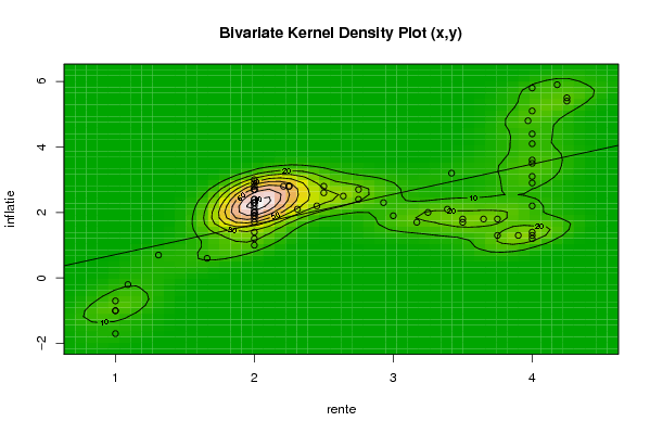
Dataset | |||||||||||||||||||||
| Dataseries X: | |||||||||||||||||||||
2 2 2 2 2 2 2 2 2 2 2 2 2 2 2 2 2 2 2 2 2 2 2 2,21 2,25 2,25 2,45 2,5 2,5 2,64 2,75 2,93 3 3,17 3,25 3,39 3,5 3,5 3,65 3,75 3,75 3,9 4 4 4 4 4 4 4 4 4 4 4 4 4,18 4,25 4,25 3,97 3,42 2,75 2,31 2 1,66 1,31 1,09 1 1 1 1 | |||||||||||||||||||||
| Dataseries Y: | |||||||||||||||||||||
1,4 1,2 1 1,7 2,4 2 2,1 2 1,8 2,7 2,3 1,9 2 2,3 2,8 2,4 2,3 2,7 2,7 2,9 3 2,2 2,3 2,8 2,8 2,8 2,2 2,6 2,8 2,5 2,4 2,3 1,9 1,7 2 2,1 1,7 1,8 1,8 1,8 1,3 1,3 1,3 1,2 1,4 2,2 2,9 3,1 3,5 3,6 4,4 4,1 5,1 5,8 5,9 5,4 5,5 4,8 3,2 2,7 2,1 1,9 0,6 0,7 -0,2 -1 -1,7 -0,7 -1 | |||||||||||||||||||||
| Dataseries Z: | |||||||||||||||||||||
0,4 1 1,7 3,1 3,3 3,1 3,5 6 5,7 4,7 4,2 3,6 4,4 2,5 -0,6 -1,9 -1,9 0,7 -0,9 -1,7 -3,1 -2,1 0,2 1,2 3,8 4 6,6 5,3 7,6 4,7 6,6 4,4 4,6 6 4,8 4 2,7 3 4,1 4 2,7 2,6 3,1 4,4 3 2 1,3 1,5 1,3 3,2 1,8 3,3 1 2,4 0,4 -0,1 1,3 -1,1 -4,4 -7,5 -12,2 -14,5 -16 -16,7 -16,3 -16,9 -15 -14,6 -14,3 | |||||||||||||||||||||
Tables (Output of Computation) | |||||||||||||||||||||
| |||||||||||||||||||||
Figures (Output of Computation) | |||||||||||||||||||||
Input Parameters & R Code | |||||||||||||||||||||
| Parameters (Session): | |||||||||||||||||||||
| par1 = 50 ; par2 = 50 ; par3 = Y ; par4 = Y ; par5 = rente ; par6 = inflatie ; par7 = industri�le productie ; | |||||||||||||||||||||
| Parameters (R input): | |||||||||||||||||||||
| par1 = 50 ; par2 = 50 ; par3 = Y ; par4 = Y ; par5 = rente ; par6 = inflatie ; par7 = industri�le productie ; par8 = ; par9 = ; par10 = ; par11 = ; par12 = ; par13 = ; par14 = ; par15 = ; par16 = ; par17 = ; par18 = ; par19 = ; par20 = ; | |||||||||||||||||||||
| R code (references can be found in the software module): | |||||||||||||||||||||
x <- array(x,dim=c(length(x),1)) | |||||||||||||||||||||