Free Statistics
of Irreproducible Research!
Description of Statistical Computation | |||||||||||||||||||||||||||||||||||||||||||||||||||||||||||||||||
|---|---|---|---|---|---|---|---|---|---|---|---|---|---|---|---|---|---|---|---|---|---|---|---|---|---|---|---|---|---|---|---|---|---|---|---|---|---|---|---|---|---|---|---|---|---|---|---|---|---|---|---|---|---|---|---|---|---|---|---|---|---|---|---|---|---|
| Author's title | |||||||||||||||||||||||||||||||||||||||||||||||||||||||||||||||||
| Author | *The author of this computation has been verified* | ||||||||||||||||||||||||||||||||||||||||||||||||||||||||||||||||
| R Software Module | rwasp_edabi.wasp | ||||||||||||||||||||||||||||||||||||||||||||||||||||||||||||||||
| Title produced by software | Bivariate Explorative Data Analysis | ||||||||||||||||||||||||||||||||||||||||||||||||||||||||||||||||
| Date of computation | Mon, 02 Nov 2009 05:55:00 -0700 | ||||||||||||||||||||||||||||||||||||||||||||||||||||||||||||||||
| Cite this page as follows | Statistical Computations at FreeStatistics.org, Office for Research Development and Education, URL https://freestatistics.org/blog/index.php?v=date/2009/Nov/02/t1257166583oip7juh3nnfae11.htm/, Retrieved Sat, 04 May 2024 05:09:21 +0000 | ||||||||||||||||||||||||||||||||||||||||||||||||||||||||||||||||
| Statistical Computations at FreeStatistics.org, Office for Research Development and Education, URL https://freestatistics.org/blog/index.php?pk=52550, Retrieved Sat, 04 May 2024 05:09:21 +0000 | |||||||||||||||||||||||||||||||||||||||||||||||||||||||||||||||||
| QR Codes: | |||||||||||||||||||||||||||||||||||||||||||||||||||||||||||||||||
|
| |||||||||||||||||||||||||||||||||||||||||||||||||||||||||||||||||
| Original text written by user: | |||||||||||||||||||||||||||||||||||||||||||||||||||||||||||||||||
| IsPrivate? | No (this computation is public) | ||||||||||||||||||||||||||||||||||||||||||||||||||||||||||||||||
| User-defined keywords | |||||||||||||||||||||||||||||||||||||||||||||||||||||||||||||||||
| Estimated Impact | 119 | ||||||||||||||||||||||||||||||||||||||||||||||||||||||||||||||||
Tree of Dependent Computations | |||||||||||||||||||||||||||||||||||||||||||||||||||||||||||||||||
| Family? (F = Feedback message, R = changed R code, M = changed R Module, P = changed Parameters, D = changed Data) | |||||||||||||||||||||||||||||||||||||||||||||||||||||||||||||||||
| - [Bivariate Explorative Data Analysis] [WS5-Bivariate EDA...] [2009-11-02 12:55:00] [0cc924834281808eda7297686c82928f] [Current] | |||||||||||||||||||||||||||||||||||||||||||||||||||||||||||||||||
| Feedback Forum | |||||||||||||||||||||||||||||||||||||||||||||||||||||||||||||||||
Post a new message | |||||||||||||||||||||||||||||||||||||||||||||||||||||||||||||||||
Dataset | |||||||||||||||||||||||||||||||||||||||||||||||||||||||||||||||||
| Dataseries X: | |||||||||||||||||||||||||||||||||||||||||||||||||||||||||||||||||
-1345.524047 -2903.542911 426.0061823 128.1400331 -360.1263768 -259.1728883 -851.6235307 469.1211691 2334.282666 -64.10234394 2157.52892 733.142615 250.1555364 -1624.55119 1808.534593 2905.586023 1848.615216 655.7679328 1162.523228 1123.254495 2741.764052 400.2289131 1425.329685 1570.489633 719.8782672 -1347.917082 745.7103047 1403.037429 546.7694751 -3489.706533 -2062.764672 -2280.596458 -1467.803967 -942.9943854 -886.3881872 -1996.031094 -727.0034212 -4770.786129 -2052.208885 82.89190751 -2652.026713 -3341.779671 -1548.248651 -2073.976825 -671.6197169 -996.3949052 -1187.367253 -2360.1001 -1662.506024 -5020.72902 -1908.497264 -118.53264 -2970.561859 -1405.816092 -1646.800071 -2214.467019 -665.0835758 -844.221019 -1508.620238 -946.0127792 -1476.407844 -2652.22204 -492.9050182 1170.670463 -1799.745861 -362.6308353 -545.7584742 -1249.361082 287.2918716 305.302748 -1730.877381 425.2830983 -804.554091 -2345.11198 1234.432456 -187.8556572 147.147942 459.244866 278.0192908 147.6453824 2533.081024 129.2296303 1944.763989 1985.781554 410.3650286 -1545.498547 146.4636974 1225.492132 958.918742 520.7373862 1099.749254 64.93192921 3521.043053 610.6412411 2210.921351 1841.389285 1973.5552 -552.013028 1098.968101 3297.288254 481.756705 995.6513386 3233.046931 3195.216694 3279.56372 5136.845895 4246.561412 4541.772999 4129.559065 617.9107561 3309.055684 3685.163193 -1679.698063 -1579.335244 -1534.49105 -2274.367558 -1549.988757 -1364.544547 -1420.58485 -195.0641937 | |||||||||||||||||||||||||||||||||||||||||||||||||||||||||||||||||
| Dataseries Y: | |||||||||||||||||||||||||||||||||||||||||||||||||||||||||||||||||
-9,950226456 -50,34292536 -6,014069555 -16,96378285 -30,80492445 38,72826771 -8,137816864 27,54351825 19,61109823 33,58231736 87,90010911 23,6982651 19,50621454 -155,5096355 -191,6906481 36,5201684 -125,4821252 -2,882323942 -88,03410605 -9,502682971 -29,73106637 -16,32715355 -56,49376266 59,23658854 56,89313054 -45,58155181 -35,39887115 -95,16443446 -32,37235783 83,251308 205,2927982 180,0921499 -52,09798504 -48,03094912 -216,5252184 -246,9460531 204,2802909 -86,90284266 -172,6419936 40,47318523 -572,696242 144,6375007 42,23202084 -243,0953917 -25,0048854 -140,55699 -198,2124341 -445,4037679 62,53645493 -129,1123364 -238,8775543 -53,8696505 -271,4195919 -38,57712427 -135,7379016 -116,4300565 -517,306661 -128,7052112 -168,687742 -387,9452614 -224,4330961 -132,0323207 -562,1477765 183,175254 -472,5757885 -169,1114404 -181,8014711 -214,515754 -245,8199438 9,420155311 -717,8145616 -246,3604598 74,80515564 87,19718014 88,97345562 186,4997702 -262,0247036 -235,8605575 292,0422345 88,25185206 86,2058235 276,188136 181,266754 142,4727584 269,3188358 310,6470922 -400,7473563 131,5714845 -423,2496727 159,4151739 394,0165162 172,920152 709,4971541 -2,788318665 218,4214259 -103,4524387 514,614897 -148,33898 495,5410584 -66,92044222 198,0749184 4,591126846 305,3890808 134,2688456 232,0912474 528,1506303 196,975153 -42,99672098 144,8522984 99,45454314 138,1478089 208,6379438 66,08000411 276,3296979 213,9395174 98,8189303 150,4010864 445,3222469 351,7020638 262,4552631 | |||||||||||||||||||||||||||||||||||||||||||||||||||||||||||||||||
Tables (Output of Computation) | |||||||||||||||||||||||||||||||||||||||||||||||||||||||||||||||||
| |||||||||||||||||||||||||||||||||||||||||||||||||||||||||||||||||
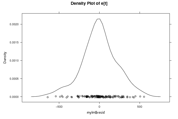
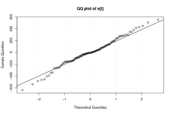
Figures (Output of Computation) | |||||||||||||||||||||||||||||||||||||||||||||||||||||||||||||||||
Input Parameters & R Code | |||||||||||||||||||||||||||||||||||||||||||||||||||||||||||||||||
| Parameters (Session): | |||||||||||||||||||||||||||||||||||||||||||||||||||||||||||||||||
| par1 = 0 ; par2 = 36 ; | |||||||||||||||||||||||||||||||||||||||||||||||||||||||||||||||||
| Parameters (R input): | |||||||||||||||||||||||||||||||||||||||||||||||||||||||||||||||||
| par1 = 0 ; par2 = 36 ; | |||||||||||||||||||||||||||||||||||||||||||||||||||||||||||||||||
| R code (references can be found in the software module): | |||||||||||||||||||||||||||||||||||||||||||||||||||||||||||||||||
par1 <- as.numeric(par1) | |||||||||||||||||||||||||||||||||||||||||||||||||||||||||||||||||