Free Statistics
of Irreproducible Research!
Description of Statistical Computation | |||||||||||||||||||||
|---|---|---|---|---|---|---|---|---|---|---|---|---|---|---|---|---|---|---|---|---|---|
| Author's title | |||||||||||||||||||||
| Author | *The author of this computation has been verified* | ||||||||||||||||||||
| R Software Module | rwasp_cloud.wasp | ||||||||||||||||||||
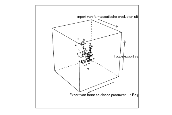
| Title produced by software | Trivariate Scatterplots | ||||||||||||||||||||
| Date of computation | Mon, 02 Nov 2009 04:33:01 -0700 | ||||||||||||||||||||
| Cite this page as follows | Statistical Computations at FreeStatistics.org, Office for Research Development and Education, URL https://freestatistics.org/blog/index.php?v=date/2009/Nov/02/t1257161814piq6jg6vfa82fj1.htm/, Retrieved Fri, 03 May 2024 21:59:31 +0000 | ||||||||||||||||||||
| Statistical Computations at FreeStatistics.org, Office for Research Development and Education, URL https://freestatistics.org/blog/index.php?pk=52496, Retrieved Fri, 03 May 2024 21:59:31 +0000 | |||||||||||||||||||||
| QR Codes: | |||||||||||||||||||||
|
| |||||||||||||||||||||
| Original text written by user: | |||||||||||||||||||||
| IsPrivate? | No (this computation is public) | ||||||||||||||||||||
| User-defined keywords | |||||||||||||||||||||
| Estimated Impact | 147 | ||||||||||||||||||||
Tree of Dependent Computations | |||||||||||||||||||||
| Family? (F = Feedback message, R = changed R code, M = changed R Module, P = changed Parameters, D = changed Data) | |||||||||||||||||||||
| - [Univariate Data Series] [De Belgische uitv...] [2009-10-13 01:35:54] [df6326eec97a6ca984a853b142930499] F PD [Univariate Data Series] [Belgische uitvoer...] [2009-10-13 07:43:28] [74be16979710d4c4e7c6647856088456] - RMPD [Trivariate Scatterplots] [WS4-Trivariate Sc...] [2009-11-02 11:33:01] [0cc924834281808eda7297686c82928f] [Current] | |||||||||||||||||||||
| Feedback Forum | |||||||||||||||||||||
Post a new message | |||||||||||||||||||||
Dataset | |||||||||||||||||||||
| Dataseries X: | |||||||||||||||||||||
11881.4 10374.2 13828 13490.5 13092.2 13184.4 12398.4 13882.3 15861.5 13286.1 15634.9 14211 13646.8 12224.6 15916.4 16535.9 15796 14418.6 15044.5 14944.2 16754.8 14254 15454.9 15644.8 14568.3 12520.2 14803 15873.2 14755.3 12875.1 14291.1 14205.3 15859.4 15258.9 15498.6 15106.5 15023.6 12083 15761.3 16943 15070.3 13659.6 14768.9 14725.1 15998.1 15370.6 14956.9 15469.7 15101.8 11703.7 16283.6 16726.5 14968.9 14861 14583.3 15305.8 17903.9 16379.4 15420.3 17870.5 15912.8 13866.5 17823.2 17872 17420.4 16704.4 15991.2 16583.6 19123.5 17838.7 17209.4 18586.5 16258.1 15141.6 19202.1 17746.5 19090.1 18040.3 17515.5 17751.8 21072.4 17170 19439.5 19795.4 17574.9 16165.4 19464.6 19932.1 19961.2 17343.4 18924.2 18574.1 21350.6 18594.6 19823.1 20844.4 19640.2 17735.4 19813.6 22160 20664.3 17877.4 20906.5 21164.1 21374.4 22952.3 21343.5 23899.3 22392.9 18274.1 22786.7 22321.5 17842.2 16373.5 15993.8 16446.1 17729 16643 16196.7 18252.1 | |||||||||||||||||||||
| Dataseries Y: | |||||||||||||||||||||
423.4 404.1 500 472.6 496.1 562 434.8 538.2 577.6 518.1 625.2 561.2 523.3 536.1 607.3 637.3 606.9 652.9 617.2 670.4 729.9 677.2 710 844.3 748.2 653.9 742.6 854.2 808.4 1819 1936.5 1966.1 2083.1 1620.1 1527.6 1795 1685.1 1851.8 2164.4 1981.8 1726.5 2144.6 1758.2 1672.9 1837.3 1596.1 1446 1898.4 1964.1 1755.9 2255.3 1881.2 2117.9 1656.5 1544.1 2098.9 2133.3 1963.5 1801.2 2365.4 1936.5 1667.6 1983.5 2058.6 2448.3 1858.1 1625.4 2130.6 2515.7 2230.2 2086.9 2235 2100.2 2288.6 2490 2573.7 2543.8 2004.7 2390 2338.4 2724.5 2292.5 2386 2477.9 2337 2605.1 2560.8 2839.3 2407.2 2085.2 2735.6 2798.7 3053.2 2405 2471.9 2727.3 2790.7 2385.4 3206.6 2705.6 3518.4 1954.9 2584.3 2535.8 2685.9 2866 2236.6 2934.9 2668.6 2371.2 3165.9 2887.2 3112.2 2671.2 2432.6 2812.3 3095.7 2862.9 2607.3 2862.5 | |||||||||||||||||||||
| Dataseries Z: | |||||||||||||||||||||
286.1 307 358.1 341.8 378.8 375.2 295.6 362.7 409.6 336.8 389.1 389.3 355.9 542 648.4 452 582.4 506.5 555.5 530.4 609.4 543.9 616.2 634.6 541.7 549.8 627.6 797.4 689.8 1576.6 1572.1 1626.4 1972.4 1509.6 1584.9 1880 1324 1777.7 2172.4 1780.3 2134.9 1838.4 1557 1755.2 1702 1577.5 1485.9 2179.1 1740.9 1724.5 2328.1 1774.1 2224.2 1536.3 1521.2 2051.8 2483.1 1929.8 1808.6 2584.9 1997.9 1639.9 2379.1 1715 2750.9 1865.4 1647.4 2180.4 2593 2057.2 2635.8 2315.4 1863.6 2038 2235.8 2222.1 2636.9 2076.8 1935.5 2086.3 2470.9 1854.6 2041.3 2170.8 1905.5 2130.2 2791.2 2539.7 2661.3 1764.9 2176.9 2458.5 2179 2242.5 2089.6 2661.6 2112 2367.3 2543 2603.9 3146.7 1789.2 2114.8 2236.3 2288.1 2173.2 1877.7 2807.4 2357.4 2107.7 2856.8 2510.8 2875 2229.7 2055.1 2545.4 2775.1 2252.2 2091.7 2433 | |||||||||||||||||||||
Tables (Output of Computation) | |||||||||||||||||||||
| |||||||||||||||||||||
Figures (Output of Computation) | |||||||||||||||||||||
Input Parameters & R Code | |||||||||||||||||||||
| Parameters (Session): | |||||||||||||||||||||
| par1 = 50 ; par2 = 50 ; par3 = Y ; par4 = Y ; par5 = Totale export van Belgi� ; par6 = Export van farmaceutische producten uit Belgi� ; par7 = Import van farmaceutische producten uit Belgi� ; | |||||||||||||||||||||
| Parameters (R input): | |||||||||||||||||||||
| par1 = 50 ; par2 = 50 ; par3 = Y ; par4 = Y ; par5 = Totale export van Belgi� ; par6 = Export van farmaceutische producten uit Belgi� ; par7 = Import van farmaceutische producten uit Belgi� ; | |||||||||||||||||||||
| R code (references can be found in the software module): | |||||||||||||||||||||
x <- array(x,dim=c(length(x),1)) | |||||||||||||||||||||