Free Statistics
of Irreproducible Research!
Description of Statistical Computation | |||||||||||||||||||||
|---|---|---|---|---|---|---|---|---|---|---|---|---|---|---|---|---|---|---|---|---|---|
| Author's title | |||||||||||||||||||||
| Author | *The author of this computation has been verified* | ||||||||||||||||||||
| R Software Module | rwasp_cloud.wasp | ||||||||||||||||||||
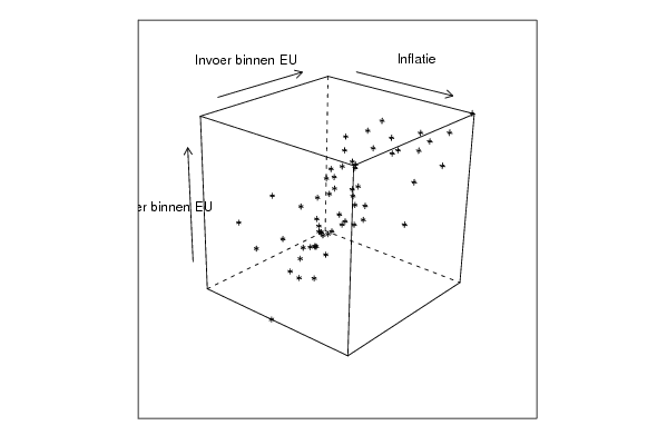
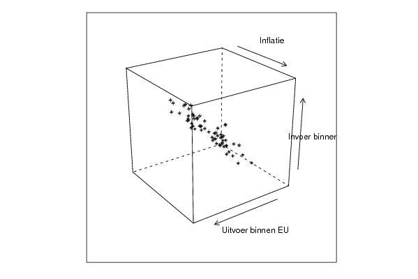
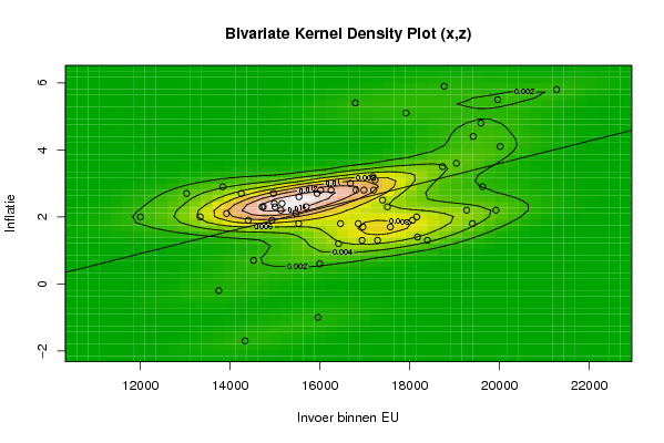
| Title produced by software | Trivariate Scatterplots | ||||||||||||||||||||
| Date of computation | Mon, 02 Nov 2009 01:08:22 -0700 | ||||||||||||||||||||
| Cite this page as follows | Statistical Computations at FreeStatistics.org, Office for Research Development and Education, URL https://freestatistics.org/blog/index.php?v=date/2009/Nov/02/t125714939803dwkucbgrmx46i.htm/, Retrieved Fri, 03 May 2024 17:31:09 +0000 | ||||||||||||||||||||
| Statistical Computations at FreeStatistics.org, Office for Research Development and Education, URL https://freestatistics.org/blog/index.php?pk=52446, Retrieved Fri, 03 May 2024 17:31:09 +0000 | |||||||||||||||||||||
| QR Codes: | |||||||||||||||||||||
|
| |||||||||||||||||||||
| Original text written by user: | |||||||||||||||||||||
| IsPrivate? | No (this computation is public) | ||||||||||||||||||||
| User-defined keywords | tri scatterplot | ||||||||||||||||||||
| Estimated Impact | 161 | ||||||||||||||||||||
Tree of Dependent Computations | |||||||||||||||||||||
| Family? (F = Feedback message, R = changed R code, M = changed R Module, P = changed Parameters, D = changed Data) | |||||||||||||||||||||
| - [Trivariate Scatterplots] [Workshop 5 - 1] [2009-10-28 20:27:13] [33b67a4fef396e07351e7d265eba4806] - MPD [Trivariate Scatterplots] [tri scatterplot] [2009-11-02 08:08:22] [950726a732ba3ca782ecb1a5307d0f6f] [Current] | |||||||||||||||||||||
| Feedback Forum | |||||||||||||||||||||
Post a new message | |||||||||||||||||||||
Dataset | |||||||||||||||||||||
| Dataseries X: | |||||||||||||||||||||
12002.4 15525.5 14247.9 15000.7 14931.4 13333.7 14711.2 17197.3 14985.2 14734.4 15937.8 13028.1 13836.8 16677.5 15130 17504 16979.9 16012.5 16247.7 19268.2 15533 16803.3 17396.1 15155.4 15692.4 18063.7 17568.6 18154.3 15467.4 16956.1 16854 19396.4 16457.6 17284.5 18395.3 16938.7 16414.3 18173.4 19919.7 19623.8 17228.1 18730.3 19039.1 19413.3 20013.6 17917.2 21270.3 18766.1 16790.8 19960.6 19586.7 17179 14964.9 13918.5 14401.3 15994.6 14521.1 13746.5 15956 14332.2 | |||||||||||||||||||||
| Dataseries Y: | |||||||||||||||||||||
13132.1 17665.9 16913 17318.8 16224.2 15469.6 16557.5 19414.8 17335 16525.2 18160.4 15553.8 15262.2 18581 17564.1 18948.6 17187.8 17564.8 17668.4 20811.7 17257.8 18984.2 20532.6 17082.3 16894.9 20274.9 20078.6 19900.9 17012.2 19642.9 19024 21691 18835.9 19873.4 21468.2 19406.8 18385.3 20739.3 22268.3 21569 17514.8 21124.7 21251 21393 22145.2 20310.5 23466.9 21264.6 18388.1 22635.4 22014.3 18422.7 16120.2 16037.7 16410.7 17749.8 16349.8 15662.3 17782.3 16398.9 | |||||||||||||||||||||
| Dataseries Z: | |||||||||||||||||||||
2 1.8 2.7 2.3 1.9 2 2.3 2.8 2.4 2.3 2.7 2.7 2.9 3 2.2 2.3 2.8 2.8 2.8 2.2 2.6 2.8 2.5 2.4 2.3 1.9 1.7 2 2.1 1.7 1.8 1.8 1.8 1.3 1.3 1.3 1.2 1.4 2.2 2.9 3.1 3.5 3.6 4.4 4.1 5.1 5.8 5.9 5.4 5.5 4.8 3.2 2.7 2.1 1.9 0.6 0.7 -0.2 -1 -1.7 | |||||||||||||||||||||
Tables (Output of Computation) | |||||||||||||||||||||
| |||||||||||||||||||||
Figures (Output of Computation) | |||||||||||||||||||||
Input Parameters & R Code | |||||||||||||||||||||
| Parameters (Session): | |||||||||||||||||||||
| par1 = 50 ; par2 = 50 ; par3 = Y ; par4 = Y ; par5 = Invoer binnen EU ; par6 = Uitvoer binnen EU ; par7 = Inflatie ; | |||||||||||||||||||||
| Parameters (R input): | |||||||||||||||||||||
| par1 = 50 ; par2 = 50 ; par3 = Y ; par4 = Y ; par5 = Invoer binnen EU ; par6 = Uitvoer binnen EU ; par7 = Inflatie ; | |||||||||||||||||||||
| R code (references can be found in the software module): | |||||||||||||||||||||
x <- array(x,dim=c(length(x),1)) | |||||||||||||||||||||