Free Statistics
of Irreproducible Research!
Description of Statistical Computation | |||||||||||||||||||||
|---|---|---|---|---|---|---|---|---|---|---|---|---|---|---|---|---|---|---|---|---|---|
| Author's title | |||||||||||||||||||||
| Author | *Unverified author* | ||||||||||||||||||||
| R Software Module | rwasp_sdplot.wasp | ||||||||||||||||||||
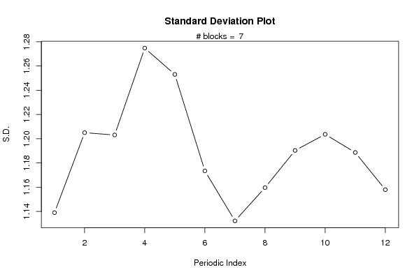
| Title produced by software | Standard Deviation Plot | ||||||||||||||||||||
| Date of computation | Wed, 27 May 2009 15:50:00 -0600 | ||||||||||||||||||||
| Cite this page as follows | Statistical Computations at FreeStatistics.org, Office for Research Development and Education, URL https://freestatistics.org/blog/index.php?v=date/2009/May/27/t12434610700zrqt4cj0c5x976.htm/, Retrieved Fri, 03 May 2024 02:39:30 +0000 | ||||||||||||||||||||
| Statistical Computations at FreeStatistics.org, Office for Research Development and Education, URL https://freestatistics.org/blog/index.php?pk=40521, Retrieved Fri, 03 May 2024 02:39:30 +0000 | |||||||||||||||||||||
| QR Codes: | |||||||||||||||||||||
|
| |||||||||||||||||||||
| Original text written by user: | |||||||||||||||||||||
| IsPrivate? | No (this computation is public) | ||||||||||||||||||||
| User-defined keywords | |||||||||||||||||||||
| Estimated Impact | 123 | ||||||||||||||||||||
Tree of Dependent Computations | |||||||||||||||||||||
| Family? (F = Feedback message, R = changed R code, M = changed R Module, P = changed Parameters, D = changed Data) | |||||||||||||||||||||
| - [Standard Deviation Plot] [standard deviatio...] [2009-01-08 20:35:37] [a18c43c8b63fa6800a53bb187b9ddd45] - D [Standard Deviation Plot] [Maxime Jonckheere...] [2009-05-27 21:50:00] [d41d8cd98f00b204e9800998ecf8427e] [Current] | |||||||||||||||||||||
| Feedback Forum | |||||||||||||||||||||
Post a new message | |||||||||||||||||||||
Dataset | |||||||||||||||||||||
| Dataseries X: | |||||||||||||||||||||
66.2 66.2 66.2 66.08 66.31 66.39 66.37 66.23 66.27 66.27 66.27 66.28 66.28 66.28 66.26 66.13 65.86 65.9 65.94 65.94 65.91 65.95 65.91 66.08 66.47 66.47 66.56 66.78 67.08 67.28 67.27 67.27 67.26 67.37 67.5 67.63 67.64 67.64 67.71 67.87 67.93 68.33 68.39 68.39 68.58 68.44 68.49 68.52 68.54 68.54 68.54 68.62 68.75 68.71 68.72 68.72 68.72 68.92 68.9 69.12 69.09 69.09 69.1 69.16 68.83 68.52 68.53 68.53 68.51 68.38 68.44 68.41 68.42 68.42 68.45 68.63 68.84 68.72 68.37 68.37 68.47 68.69 68.46 68.17 68.17 | |||||||||||||||||||||
Tables (Output of Computation) | |||||||||||||||||||||
| |||||||||||||||||||||
Figures (Output of Computation) | |||||||||||||||||||||
Input Parameters & R Code | |||||||||||||||||||||
| Parameters (Session): | |||||||||||||||||||||
| par1 = 12 ; | |||||||||||||||||||||
| Parameters (R input): | |||||||||||||||||||||
| par1 = 12 ; | |||||||||||||||||||||
| R code (references can be found in the software module): | |||||||||||||||||||||
par1 <- as.numeric(par1) | |||||||||||||||||||||