Free Statistics
of Irreproducible Research!
Description of Statistical Computation | |||||||||||||||||||||||||||||||||||||||||||||||||||||||||||||||||||||||||||||||||||||
|---|---|---|---|---|---|---|---|---|---|---|---|---|---|---|---|---|---|---|---|---|---|---|---|---|---|---|---|---|---|---|---|---|---|---|---|---|---|---|---|---|---|---|---|---|---|---|---|---|---|---|---|---|---|---|---|---|---|---|---|---|---|---|---|---|---|---|---|---|---|---|---|---|---|---|---|---|---|---|---|---|---|---|---|---|---|
| Author's title | |||||||||||||||||||||||||||||||||||||||||||||||||||||||||||||||||||||||||||||||||||||
| Author | *Unverified author* | ||||||||||||||||||||||||||||||||||||||||||||||||||||||||||||||||||||||||||||||||||||
| R Software Module | rwasp_bootstrapplot.wasp | ||||||||||||||||||||||||||||||||||||||||||||||||||||||||||||||||||||||||||||||||||||
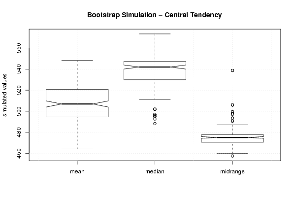
| Title produced by software | Blocked Bootstrap Plot - Central Tendency | ||||||||||||||||||||||||||||||||||||||||||||||||||||||||||||||||||||||||||||||||||||
| Date of computation | Sun, 17 May 2009 05:08:11 -0600 | ||||||||||||||||||||||||||||||||||||||||||||||||||||||||||||||||||||||||||||||||||||
| Cite this page as follows | Statistical Computations at FreeStatistics.org, Office for Research Development and Education, URL https://freestatistics.org/blog/index.php?v=date/2009/May/17/t1242558592sf47cbwagg3zuly.htm/, Retrieved Fri, 03 May 2024 22:33:25 +0000 | ||||||||||||||||||||||||||||||||||||||||||||||||||||||||||||||||||||||||||||||||||||
| Statistical Computations at FreeStatistics.org, Office for Research Development and Education, URL https://freestatistics.org/blog/index.php?pk=40195, Retrieved Fri, 03 May 2024 22:33:25 +0000 | |||||||||||||||||||||||||||||||||||||||||||||||||||||||||||||||||||||||||||||||||||||
| QR Codes: | |||||||||||||||||||||||||||||||||||||||||||||||||||||||||||||||||||||||||||||||||||||
|
| |||||||||||||||||||||||||||||||||||||||||||||||||||||||||||||||||||||||||||||||||||||
| Original text written by user: | |||||||||||||||||||||||||||||||||||||||||||||||||||||||||||||||||||||||||||||||||||||
| IsPrivate? | No (this computation is public) | ||||||||||||||||||||||||||||||||||||||||||||||||||||||||||||||||||||||||||||||||||||
| User-defined keywords | |||||||||||||||||||||||||||||||||||||||||||||||||||||||||||||||||||||||||||||||||||||
| Estimated Impact | 184 | ||||||||||||||||||||||||||||||||||||||||||||||||||||||||||||||||||||||||||||||||||||
Tree of Dependent Computations | |||||||||||||||||||||||||||||||||||||||||||||||||||||||||||||||||||||||||||||||||||||
| Family? (F = Feedback message, R = changed R code, M = changed R Module, P = changed Parameters, D = changed Data) | |||||||||||||||||||||||||||||||||||||||||||||||||||||||||||||||||||||||||||||||||||||
| - [Blocked Bootstrap Plot - Central Tendency] [Kempeneers Liesbe...] [2009-05-17 11:08:11] [866e757444a60b1c09d57e14cc8533e4] [Current] - PD [Blocked Bootstrap Plot - Central Tendency] [] [2009-06-02 16:19:42] [74be16979710d4c4e7c6647856088456] - PD [Blocked Bootstrap Plot - Central Tendency] [Yelle Eyckmans] [2009-06-06 10:41:06] [74be16979710d4c4e7c6647856088456] - PD [Blocked Bootstrap Plot - Central Tendency] [Yelle Eyckmans] [2009-06-06 10:43:02] [74be16979710d4c4e7c6647856088456] - P [Blocked Bootstrap Plot - Central Tendency] [Yelle Eyckmans] [2009-06-06 10:44:49] [74be16979710d4c4e7c6647856088456] - PD [Blocked Bootstrap Plot - Central Tendency] [] [2009-06-02 16:25:07] [74be16979710d4c4e7c6647856088456] | |||||||||||||||||||||||||||||||||||||||||||||||||||||||||||||||||||||||||||||||||||||
| Feedback Forum | |||||||||||||||||||||||||||||||||||||||||||||||||||||||||||||||||||||||||||||||||||||
Post a new message | |||||||||||||||||||||||||||||||||||||||||||||||||||||||||||||||||||||||||||||||||||||
Dataset | |||||||||||||||||||||||||||||||||||||||||||||||||||||||||||||||||||||||||||||||||||||
| Dataseries X: | |||||||||||||||||||||||||||||||||||||||||||||||||||||||||||||||||||||||||||||||||||||
196.9 192.1 201.8 186.9 218.0 214.4 227.5 204.1 225.8 223.7 244.7 243.9 257.3 234.5 251.4 243.8 247.4 245.3 262.5 270.0 259.9 262.2 244.9 249.3 268.2 231.2 264.3 252.7 275.5 261.5 275.5 272.3 268.6 270.4 267.7 275.0 272.6 248.6 279.4 270.5 292.8 297.8 296.8 290.9 282.8 312.8 303.2 301.4 289.8 279.6 302.2 299.1 319.7 310.9 315.2 338.5 315.6 321.2 318.5 342.7 261.4 287.0 331.5 326.9 338.6 337.0 358.4 344.5 345.7 344.1 317.4 354.5 345.2 314.1 352.5 361.2 365.9 332.5 364.0 359.1 345.6 366.9 370.2 359.9 366.6 336.3 368.5 374.2 384.3 358.9 407.7 433.3 404.7 392.7 409.7 416.5 414.3 404.3 421.4 372.6 404.7 420.2 438.4 449.1 445.8 413.8 420.5 442.3 438.9 394.5 416.8 402.9 424.5 432.3 484.1 492.7 496.3 471.9 491.2 512.9 482.4 407.9 448.5 431.1 498.8 497.1 517.1 487.7 512.5 550.1 532.5 524.1 515.7 461.0 529.3 467.4 559.8 536.5 531.9 546.5 547.4 536.1 482.8 551.0 532.9 484.1 554.8 537.0 558.0 511.4 502.9 558.6 545.1 574.3 542.2 600.0 588.6 524.4 618.5 580.9 557.2 571.2 597.5 601.7 558.9 600.9 601.0 615.7 578.1 495.9 526.8 522.1 605.1 574.4 609.7 580.7 565.1 590.7 571.5 601.3 567.3 467.9 588.9 579.4 502.6 568.7 616.0 586.2 575.5 599.9 568.2 516.0 493.4 496.8 529.9 491.7 543.2 490.8 554.7 625.7 605.0 645.2 645.2 611.8 600.3 549.8 635.5 617.7 643.5 485.7 689.5 692.0 677.3 704.7 668.6 717.8 689.8 640.4 675.2 528.1 538.0 527.2 655.6 650.6 623.7 748.4 727.4 750.5 678.9 659.5 691.9 639.8 663.8 572.9 592.5 734.8 696.1 589.2 662.9 661.2 672.1 583.7 705.5 631.0 733.3 674.9 695.5 634.1 630.6 635.2 554.1 623.9 679.3 565.6 564.1 637.2 650.8 602.7 587.5 619.2 616.5 637.9 557.9 594.0 668.7 603.3 674.5 573.4 706.0 693.7 627.5 550.7 592.3 660.2 597.3 641.0 663.6 595.9 638.4 665.4 671.4 637.0 685.7 705.8 704.8 734.4 674.2 748.6 763.4 658.0 627.5 528.9 488.3 575.5 735.6 685.3 613.6 629.5 634.7 652.6 728.3 634.3 690.7 676.3 675.4 595.6 712.4 735.8 544.4 567.0 510.0 564.0 630.7 496.7 660.9 601.2 655.2 591.6 606.1 560.7 368.3 371.6 413.9 413.9 389.0 399.2 429.8 395.6 472 486 525 396 511 525 492 517 525 474 539 468 543 532 565 535 534 546 494 552 511 451 537 494 549 544 598 583 582 589 578 561 592 504 545 547 585 562 520 581 590 562 548 567 542 473 531 462 479 533 552 547 562 524 479 445 406 475 589 495 484 536 555 565 564 573 569 588 546 508 560 558 516 549 595 586 597 592 538 590 576 451 538 555 532 530 553 626 601 573 569 562 468 483 460 411 458 455 600 605 545 549 415 568 577 517 558 518 489 502 569 540 550 557 542 542 582 525 584 562 639 613 604 613 625 654 638 | |||||||||||||||||||||||||||||||||||||||||||||||||||||||||||||||||||||||||||||||||||||
Tables (Output of Computation) | |||||||||||||||||||||||||||||||||||||||||||||||||||||||||||||||||||||||||||||||||||||
| |||||||||||||||||||||||||||||||||||||||||||||||||||||||||||||||||||||||||||||||||||||
Figures (Output of Computation) | |||||||||||||||||||||||||||||||||||||||||||||||||||||||||||||||||||||||||||||||||||||
Input Parameters & R Code | |||||||||||||||||||||||||||||||||||||||||||||||||||||||||||||||||||||||||||||||||||||
| Parameters (Session): | |||||||||||||||||||||||||||||||||||||||||||||||||||||||||||||||||||||||||||||||||||||
| par1 = 200 ; par2 = 12 ; | |||||||||||||||||||||||||||||||||||||||||||||||||||||||||||||||||||||||||||||||||||||
| Parameters (R input): | |||||||||||||||||||||||||||||||||||||||||||||||||||||||||||||||||||||||||||||||||||||
| par1 = 200 ; par2 = 12 ; | |||||||||||||||||||||||||||||||||||||||||||||||||||||||||||||||||||||||||||||||||||||
| R code (references can be found in the software module): | |||||||||||||||||||||||||||||||||||||||||||||||||||||||||||||||||||||||||||||||||||||
par1 <- as.numeric(par1) | |||||||||||||||||||||||||||||||||||||||||||||||||||||||||||||||||||||||||||||||||||||