Repository of Reproducible Computations

Free Statistics

of Irreproducible Research!

Author's title

Author

*Unverified author*

R Software Module

rwasp_autocorrelation.wasp

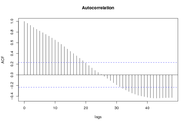
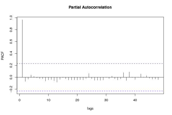
Title produced by software

(Partial) Autocorrelation Function

Date of computation

Thu, 14 May 2009 16:31:44 -0600

Cite this page as follows

Statistical Computations at FreeStatistics.org, Office for Research Development and Education, URL https://freestatistics.org/blog/index.php?v=date/2009/May/15/t12423403655axpbow0y9mvxka.htm/, Retrieved Mon, 29 Apr 2024 18:19:37 +0000

Statistical Computations at FreeStatistics.org, Office for Research Development and Education, URL https://freestatistics.org/blog/index.php?pk=40116, Retrieved Mon, 29 Apr 2024 18:19:37 +0000

QR Codes:

Paste this QR Code to cite your computation.

Original text written by user:

IsPrivate?

No (this computation is public)

User-defined keywords

Estimated Impact

158

Family? (F = Feedback message, R = changed R code, M = changed R Module, P = changed Parameters, D = changed Data)

-       [(Partial) Autocorrelation Function] [Time Series analy...] [2009-05-14 22:31:44] [2f928979fcb5db36e984611041f4b2ce] [Current]

Feedback Forum

Post a new message

Dataseries X:

Download CSV

Histogram

Boxplots

2,98
2,98
2,98
3,03
3,07
3,08
3,08
3,08
3,08
3,08
3,08
3,08
3,08
3,08
3,12
3,15
3,15
3,15
3,15
3,16
3,19
3,2
3,2
3,2
3,21
3,21
3,21
3,21
3,21
3,28
3,3
3,3
3,3
3,3
3,3
3,3
3,3
3,45
3,49
3,5
3,54
3,64
3,67
3,67
3,68
3,68
3,68
3,68
3,7
3,83
3,87
3,87
3,87
3,87
3,87
3,87
3,87
3,87
3,87
3,88
3,88
3,88
3,88
3,88
3,88
3,89
3,89
3,91
3,95
3,99
3,99
3,99

Summary of computational transaction
Raw Input	view raw input (R code)
Raw Output	view raw output of R engine
Computing time	1 seconds
R Server	'Gwilym Jenkins' @ 72.249.127.135

\begin{tabular}{lllllllll}
\hline
Summary of computational transaction \tabularnewline
Raw Input & view raw input (R code)  \tabularnewline
Raw Output & view raw output of R engine  \tabularnewline
Computing time & 1 seconds \tabularnewline
R Server & 'Gwilym Jenkins' @ 72.249.127.135 \tabularnewline
\hline
\end{tabular}
%Source: https://freestatistics.org/blog/index.php?pk=40116&T=0

[TABLE]
[ROW][C]Summary of computational transaction[/C][/ROW]
[ROW][C]Raw Input[/C][C]view raw input (R code) [/C][/ROW]
[ROW][C]Raw Output[/C][C]view raw output of R engine [/C][/ROW]
[ROW][C]Computing time[/C][C]1 seconds[/C][/ROW]
[ROW][C]R Server[/C][C]'Gwilym Jenkins' @ 72.249.127.135[/C][/ROW]
[/TABLE]
Source: https://freestatistics.org/blog/index.php?pk=40116&T=0

Globally Unique Identifier (entire table): ba.freestatistics.org/blog/index.php?pk=40116&T=0

As an alternative you can also use a QR Code:

The GUIDs for individual cells are displayed in the table below:

Summary of computational transaction
Raw Input	view raw input (R code)
Raw Output	view raw output of R engine
Computing time	1 seconds
R Server	'Gwilym Jenkins' @ 72.249.127.135

Autocorrelation Function
Time lag k	ACF(k)	T-STAT	P-value
1	0.965511	8.1926	0
2	0.927521	7.8703	0
3	0.888585	7.5399	0
4	0.85361	7.2431	0
5	0.821308	6.969	0
6	0.789871	6.7023	0
7	0.758054	6.4323	0
8	0.725577	6.1567	0
9	0.689882	5.8538	0
10	0.652272	5.5347	0
11	0.613419	5.205	1e-06
12	0.572556	4.8583	3e-06
13	0.528122	4.4813	1.4e-05
14	0.483168	4.0998	5.4e-05
15	0.440197	3.7352	0.000186
16	0.398324	3.3799	0.000587
17	0.355765	3.0188	0.001754
18	0.31213	2.6485	0.004964
19	0.267407	2.269	0.013132
20	0.221748	1.8816	0.031967
21	0.175603	1.49	0.070291
22	0.129054	1.0951	0.13857
23	0.084034	0.7131	0.239058
24	0.046062	0.3908	0.348531
25	0.009368	0.0795	0.468432
26	-0.028201	-0.2393	0.405778
27	-0.067261	-0.5707	0.284981
28	-0.107799	-0.9147	0.181701
29	-0.148951	-1.2639	0.105174
30	-0.186974	-1.5865	0.058501
31	-0.22301	-1.8923	0.031236
32	-0.253834	-2.1539	0.0173
33	-0.283082	-2.402	0.009443
34	-0.312542	-2.652	0.004918
35	-0.341182	-2.895	0.002508
36	-0.361709	-3.0692	0.001513
37	-0.382874	-3.2488	0.000881
38	-0.396152	-3.3615	0.000622
39	-0.40812	-3.463	0.000451
40	-0.42016	-3.5652	0.000325
41	-0.430276	-3.651	0.000246
42	-0.434675	-3.6883	0.000217
43	-0.436107	-3.7005	0.000209
44	-0.433276	-3.6765	0.000226
45	-0.430209	-3.6504	0.000246
46	-0.428052	-3.6321	0.000262
47	-0.426889	-3.6223	0.00027
48	-0.426081	-3.6154	0.000276

\begin{tabular}{lllllllll}
\hline
Autocorrelation Function \tabularnewline
Time lag k & ACF(k) & T-STAT & P-value \tabularnewline
1 & 0.965511 & 8.1926 & 0 \tabularnewline
2 & 0.927521 & 7.8703 & 0 \tabularnewline
3 & 0.888585 & 7.5399 & 0 \tabularnewline
4 & 0.85361 & 7.2431 & 0 \tabularnewline
5 & 0.821308 & 6.969 & 0 \tabularnewline
6 & 0.789871 & 6.7023 & 0 \tabularnewline
7 & 0.758054 & 6.4323 & 0 \tabularnewline
8 & 0.725577 & 6.1567 & 0 \tabularnewline
9 & 0.689882 & 5.8538 & 0 \tabularnewline
10 & 0.652272 & 5.5347 & 0 \tabularnewline
11 & 0.613419 & 5.205 & 1e-06 \tabularnewline
12 & 0.572556 & 4.8583 & 3e-06 \tabularnewline
13 & 0.528122 & 4.4813 & 1.4e-05 \tabularnewline
14 & 0.483168 & 4.0998 & 5.4e-05 \tabularnewline
15 & 0.440197 & 3.7352 & 0.000186 \tabularnewline
16 & 0.398324 & 3.3799 & 0.000587 \tabularnewline
17 & 0.355765 & 3.0188 & 0.001754 \tabularnewline
18 & 0.31213 & 2.6485 & 0.004964 \tabularnewline
19 & 0.267407 & 2.269 & 0.013132 \tabularnewline
20 & 0.221748 & 1.8816 & 0.031967 \tabularnewline
21 & 0.175603 & 1.49 & 0.070291 \tabularnewline
22 & 0.129054 & 1.0951 & 0.13857 \tabularnewline
23 & 0.084034 & 0.7131 & 0.239058 \tabularnewline
24 & 0.046062 & 0.3908 & 0.348531 \tabularnewline
25 & 0.009368 & 0.0795 & 0.468432 \tabularnewline
26 & -0.028201 & -0.2393 & 0.405778 \tabularnewline
27 & -0.067261 & -0.5707 & 0.284981 \tabularnewline
28 & -0.107799 & -0.9147 & 0.181701 \tabularnewline
29 & -0.148951 & -1.2639 & 0.105174 \tabularnewline
30 & -0.186974 & -1.5865 & 0.058501 \tabularnewline
31 & -0.22301 & -1.8923 & 0.031236 \tabularnewline
32 & -0.253834 & -2.1539 & 0.0173 \tabularnewline
33 & -0.283082 & -2.402 & 0.009443 \tabularnewline
34 & -0.312542 & -2.652 & 0.004918 \tabularnewline
35 & -0.341182 & -2.895 & 0.002508 \tabularnewline
36 & -0.361709 & -3.0692 & 0.001513 \tabularnewline
37 & -0.382874 & -3.2488 & 0.000881 \tabularnewline
38 & -0.396152 & -3.3615 & 0.000622 \tabularnewline
39 & -0.40812 & -3.463 & 0.000451 \tabularnewline
40 & -0.42016 & -3.5652 & 0.000325 \tabularnewline
41 & -0.430276 & -3.651 & 0.000246 \tabularnewline
42 & -0.434675 & -3.6883 & 0.000217 \tabularnewline
43 & -0.436107 & -3.7005 & 0.000209 \tabularnewline
44 & -0.433276 & -3.6765 & 0.000226 \tabularnewline
45 & -0.430209 & -3.6504 & 0.000246 \tabularnewline
46 & -0.428052 & -3.6321 & 0.000262 \tabularnewline
47 & -0.426889 & -3.6223 & 0.00027 \tabularnewline
48 & -0.426081 & -3.6154 & 0.000276 \tabularnewline
\hline
\end{tabular}
%Source: https://freestatistics.org/blog/index.php?pk=40116&T=1

[TABLE]
[ROW][C]Autocorrelation Function[/C][/ROW]
[ROW][C]Time lag k[/C][C]ACF(k)[/C][C]T-STAT[/C][C]P-value[/C][/ROW]
[ROW][C]1[/C][C]0.965511[/C][C]8.1926[/C][C]0[/C][/ROW]
[ROW][C]2[/C][C]0.927521[/C][C]7.8703[/C][C]0[/C][/ROW]
[ROW][C]3[/C][C]0.888585[/C][C]7.5399[/C][C]0[/C][/ROW]
[ROW][C]4[/C][C]0.85361[/C][C]7.2431[/C][C]0[/C][/ROW]
[ROW][C]5[/C][C]0.821308[/C][C]6.969[/C][C]0[/C][/ROW]
[ROW][C]6[/C][C]0.789871[/C][C]6.7023[/C][C]0[/C][/ROW]
[ROW][C]7[/C][C]0.758054[/C][C]6.4323[/C][C]0[/C][/ROW]
[ROW][C]8[/C][C]0.725577[/C][C]6.1567[/C][C]0[/C][/ROW]
[ROW][C]9[/C][C]0.689882[/C][C]5.8538[/C][C]0[/C][/ROW]
[ROW][C]10[/C][C]0.652272[/C][C]5.5347[/C][C]0[/C][/ROW]
[ROW][C]11[/C][C]0.613419[/C][C]5.205[/C][C]1e-06[/C][/ROW]
[ROW][C]12[/C][C]0.572556[/C][C]4.8583[/C][C]3e-06[/C][/ROW]
[ROW][C]13[/C][C]0.528122[/C][C]4.4813[/C][C]1.4e-05[/C][/ROW]
[ROW][C]14[/C][C]0.483168[/C][C]4.0998[/C][C]5.4e-05[/C][/ROW]
[ROW][C]15[/C][C]0.440197[/C][C]3.7352[/C][C]0.000186[/C][/ROW]
[ROW][C]16[/C][C]0.398324[/C][C]3.3799[/C][C]0.000587[/C][/ROW]
[ROW][C]17[/C][C]0.355765[/C][C]3.0188[/C][C]0.001754[/C][/ROW]
[ROW][C]18[/C][C]0.31213[/C][C]2.6485[/C][C]0.004964[/C][/ROW]
[ROW][C]19[/C][C]0.267407[/C][C]2.269[/C][C]0.013132[/C][/ROW]
[ROW][C]20[/C][C]0.221748[/C][C]1.8816[/C][C]0.031967[/C][/ROW]
[ROW][C]21[/C][C]0.175603[/C][C]1.49[/C][C]0.070291[/C][/ROW]
[ROW][C]22[/C][C]0.129054[/C][C]1.0951[/C][C]0.13857[/C][/ROW]
[ROW][C]23[/C][C]0.084034[/C][C]0.7131[/C][C]0.239058[/C][/ROW]
[ROW][C]24[/C][C]0.046062[/C][C]0.3908[/C][C]0.348531[/C][/ROW]
[ROW][C]25[/C][C]0.009368[/C][C]0.0795[/C][C]0.468432[/C][/ROW]
[ROW][C]26[/C][C]-0.028201[/C][C]-0.2393[/C][C]0.405778[/C][/ROW]
[ROW][C]27[/C][C]-0.067261[/C][C]-0.5707[/C][C]0.284981[/C][/ROW]
[ROW][C]28[/C][C]-0.107799[/C][C]-0.9147[/C][C]0.181701[/C][/ROW]
[ROW][C]29[/C][C]-0.148951[/C][C]-1.2639[/C][C]0.105174[/C][/ROW]
[ROW][C]30[/C][C]-0.186974[/C][C]-1.5865[/C][C]0.058501[/C][/ROW]
[ROW][C]31[/C][C]-0.22301[/C][C]-1.8923[/C][C]0.031236[/C][/ROW]
[ROW][C]32[/C][C]-0.253834[/C][C]-2.1539[/C][C]0.0173[/C][/ROW]
[ROW][C]33[/C][C]-0.283082[/C][C]-2.402[/C][C]0.009443[/C][/ROW]
[ROW][C]34[/C][C]-0.312542[/C][C]-2.652[/C][C]0.004918[/C][/ROW]
[ROW][C]35[/C][C]-0.341182[/C][C]-2.895[/C][C]0.002508[/C][/ROW]
[ROW][C]36[/C][C]-0.361709[/C][C]-3.0692[/C][C]0.001513[/C][/ROW]
[ROW][C]37[/C][C]-0.382874[/C][C]-3.2488[/C][C]0.000881[/C][/ROW]
[ROW][C]38[/C][C]-0.396152[/C][C]-3.3615[/C][C]0.000622[/C][/ROW]
[ROW][C]39[/C][C]-0.40812[/C][C]-3.463[/C][C]0.000451[/C][/ROW]
[ROW][C]40[/C][C]-0.42016[/C][C]-3.5652[/C][C]0.000325[/C][/ROW]
[ROW][C]41[/C][C]-0.430276[/C][C]-3.651[/C][C]0.000246[/C][/ROW]
[ROW][C]42[/C][C]-0.434675[/C][C]-3.6883[/C][C]0.000217[/C][/ROW]
[ROW][C]43[/C][C]-0.436107[/C][C]-3.7005[/C][C]0.000209[/C][/ROW]
[ROW][C]44[/C][C]-0.433276[/C][C]-3.6765[/C][C]0.000226[/C][/ROW]
[ROW][C]45[/C][C]-0.430209[/C][C]-3.6504[/C][C]0.000246[/C][/ROW]
[ROW][C]46[/C][C]-0.428052[/C][C]-3.6321[/C][C]0.000262[/C][/ROW]
[ROW][C]47[/C][C]-0.426889[/C][C]-3.6223[/C][C]0.00027[/C][/ROW]
[ROW][C]48[/C][C]-0.426081[/C][C]-3.6154[/C][C]0.000276[/C][/ROW]
[/TABLE]
Source: https://freestatistics.org/blog/index.php?pk=40116&T=1

Globally Unique Identifier (entire table): ba.freestatistics.org/blog/index.php?pk=40116&T=1

As an alternative you can also use a QR Code:

The GUIDs for individual cells are displayed in the table below:

Autocorrelation Function
Time lag k	ACF(k)	T-STAT	P-value
1	0.965511	8.1926	0
2	0.927521	7.8703	0
3	0.888585	7.5399	0
4	0.85361	7.2431	0
5	0.821308	6.969	0
6	0.789871	6.7023	0
7	0.758054	6.4323	0
8	0.725577	6.1567	0
9	0.689882	5.8538	0
10	0.652272	5.5347	0
11	0.613419	5.205	1e-06
12	0.572556	4.8583	3e-06
13	0.528122	4.4813	1.4e-05
14	0.483168	4.0998	5.4e-05
15	0.440197	3.7352	0.000186
16	0.398324	3.3799	0.000587
17	0.355765	3.0188	0.001754
18	0.31213	2.6485	0.004964
19	0.267407	2.269	0.013132
20	0.221748	1.8816	0.031967
21	0.175603	1.49	0.070291
22	0.129054	1.0951	0.13857
23	0.084034	0.7131	0.239058
24	0.046062	0.3908	0.348531
25	0.009368	0.0795	0.468432
26	-0.028201	-0.2393	0.405778
27	-0.067261	-0.5707	0.284981
28	-0.107799	-0.9147	0.181701
29	-0.148951	-1.2639	0.105174
30	-0.186974	-1.5865	0.058501
31	-0.22301	-1.8923	0.031236
32	-0.253834	-2.1539	0.0173
33	-0.283082	-2.402	0.009443
34	-0.312542	-2.652	0.004918
35	-0.341182	-2.895	0.002508
36	-0.361709	-3.0692	0.001513
37	-0.382874	-3.2488	0.000881
38	-0.396152	-3.3615	0.000622
39	-0.40812	-3.463	0.000451
40	-0.42016	-3.5652	0.000325
41	-0.430276	-3.651	0.000246
42	-0.434675	-3.6883	0.000217
43	-0.436107	-3.7005	0.000209
44	-0.433276	-3.6765	0.000226
45	-0.430209	-3.6504	0.000246
46	-0.428052	-3.6321	0.000262
47	-0.426889	-3.6223	0.00027
48	-0.426081	-3.6154	0.000276

Partial Autocorrelation Function
Time lag k	PACF(k)	T-STAT	P-value
1	0.965511	8.1926	0
2	-0.069188	-0.5871	0.279492
3	-0.031199	-0.2647	0.395986
4	0.039382	0.3342	0.369613
5	0.015143	0.1285	0.449059
6	-0.010318	-0.0876	0.465237
7	-0.022183	-0.1882	0.425615
8	-0.0238	-0.202	0.420262
9	-0.063411	-0.5381	0.296098
10	-0.04481	-0.3802	0.35245
11	-0.038341	-0.3253	0.372935
12	-0.057377	-0.4869	0.313917
13	-0.082626	-0.7011	0.242748
14	-0.03643	-0.3091	0.379064
15	-0.003907	-0.0332	0.486823
16	-0.024411	-0.2071	0.418244
17	-0.046061	-0.3908	0.348533
18	-0.043776	-0.3714	0.355697
19	-0.043467	-0.3688	0.35667
20	-0.045324	-0.3846	0.350839
21	-0.040636	-0.3448	0.365622
22	-0.044727	-0.3795	0.352708
23	-0.020808	-0.1766	0.430174
24	0.063309	0.5372	0.296394
25	-0.023928	-0.203	0.41984
26	-0.051288	-0.4352	0.332363
27	-0.048871	-0.4147	0.339804
28	-0.051537	-0.4373	0.3316
29	-0.046966	-0.3985	0.345714
30	0.002809	0.0238	0.490524
31	-0.022131	-0.1878	0.425785
32	0.020941	0.1777	0.429732
33	-0.024796	-0.2104	0.416974
34	-0.045178	-0.3834	0.351295
35	-0.026875	-0.228	0.410128
36	0.078744	0.6682	0.253081
37	-0.054347	-0.4612	0.32304
38	0.089655	0.7608	0.224645
39	-0.003788	-0.0321	0.487224
40	-0.037258	-0.3161	0.376403
41	0.002525	0.0214	0.491483
42	0.056598	0.4802	0.316253
43	0.004164	0.0353	0.485958
44	0.027266	0.2314	0.408845
45	-0.016331	-0.1386	0.445088
46	-0.031518	-0.2674	0.394948
47	-0.02925	-0.2482	0.402345
48	-0.039613	-0.3361	0.368876

\begin{tabular}{lllllllll}
\hline
Partial Autocorrelation Function \tabularnewline
Time lag k & PACF(k) & T-STAT & P-value \tabularnewline
1 & 0.965511 & 8.1926 & 0 \tabularnewline
2 & -0.069188 & -0.5871 & 0.279492 \tabularnewline
3 & -0.031199 & -0.2647 & 0.395986 \tabularnewline
4 & 0.039382 & 0.3342 & 0.369613 \tabularnewline
5 & 0.015143 & 0.1285 & 0.449059 \tabularnewline
6 & -0.010318 & -0.0876 & 0.465237 \tabularnewline
7 & -0.022183 & -0.1882 & 0.425615 \tabularnewline
8 & -0.0238 & -0.202 & 0.420262 \tabularnewline
9 & -0.063411 & -0.5381 & 0.296098 \tabularnewline
10 & -0.04481 & -0.3802 & 0.35245 \tabularnewline
11 & -0.038341 & -0.3253 & 0.372935 \tabularnewline
12 & -0.057377 & -0.4869 & 0.313917 \tabularnewline
13 & -0.082626 & -0.7011 & 0.242748 \tabularnewline
14 & -0.03643 & -0.3091 & 0.379064 \tabularnewline
15 & -0.003907 & -0.0332 & 0.486823 \tabularnewline
16 & -0.024411 & -0.2071 & 0.418244 \tabularnewline
17 & -0.046061 & -0.3908 & 0.348533 \tabularnewline
18 & -0.043776 & -0.3714 & 0.355697 \tabularnewline
19 & -0.043467 & -0.3688 & 0.35667 \tabularnewline
20 & -0.045324 & -0.3846 & 0.350839 \tabularnewline
21 & -0.040636 & -0.3448 & 0.365622 \tabularnewline
22 & -0.044727 & -0.3795 & 0.352708 \tabularnewline
23 & -0.020808 & -0.1766 & 0.430174 \tabularnewline
24 & 0.063309 & 0.5372 & 0.296394 \tabularnewline
25 & -0.023928 & -0.203 & 0.41984 \tabularnewline
26 & -0.051288 & -0.4352 & 0.332363 \tabularnewline
27 & -0.048871 & -0.4147 & 0.339804 \tabularnewline
28 & -0.051537 & -0.4373 & 0.3316 \tabularnewline
29 & -0.046966 & -0.3985 & 0.345714 \tabularnewline
30 & 0.002809 & 0.0238 & 0.490524 \tabularnewline
31 & -0.022131 & -0.1878 & 0.425785 \tabularnewline
32 & 0.020941 & 0.1777 & 0.429732 \tabularnewline
33 & -0.024796 & -0.2104 & 0.416974 \tabularnewline
34 & -0.045178 & -0.3834 & 0.351295 \tabularnewline
35 & -0.026875 & -0.228 & 0.410128 \tabularnewline
36 & 0.078744 & 0.6682 & 0.253081 \tabularnewline
37 & -0.054347 & -0.4612 & 0.32304 \tabularnewline
38 & 0.089655 & 0.7608 & 0.224645 \tabularnewline
39 & -0.003788 & -0.0321 & 0.487224 \tabularnewline
40 & -0.037258 & -0.3161 & 0.376403 \tabularnewline
41 & 0.002525 & 0.0214 & 0.491483 \tabularnewline
42 & 0.056598 & 0.4802 & 0.316253 \tabularnewline
43 & 0.004164 & 0.0353 & 0.485958 \tabularnewline
44 & 0.027266 & 0.2314 & 0.408845 \tabularnewline
45 & -0.016331 & -0.1386 & 0.445088 \tabularnewline
46 & -0.031518 & -0.2674 & 0.394948 \tabularnewline
47 & -0.02925 & -0.2482 & 0.402345 \tabularnewline
48 & -0.039613 & -0.3361 & 0.368876 \tabularnewline
\hline
\end{tabular}
%Source: https://freestatistics.org/blog/index.php?pk=40116&T=2

[TABLE]
[ROW][C]Partial Autocorrelation Function[/C][/ROW]
[ROW][C]Time lag k[/C][C]PACF(k)[/C][C]T-STAT[/C][C]P-value[/C][/ROW]
[ROW][C]1[/C][C]0.965511[/C][C]8.1926[/C][C]0[/C][/ROW]
[ROW][C]2[/C][C]-0.069188[/C][C]-0.5871[/C][C]0.279492[/C][/ROW]
[ROW][C]3[/C][C]-0.031199[/C][C]-0.2647[/C][C]0.395986[/C][/ROW]
[ROW][C]4[/C][C]0.039382[/C][C]0.3342[/C][C]0.369613[/C][/ROW]
[ROW][C]5[/C][C]0.015143[/C][C]0.1285[/C][C]0.449059[/C][/ROW]
[ROW][C]6[/C][C]-0.010318[/C][C]-0.0876[/C][C]0.465237[/C][/ROW]
[ROW][C]7[/C][C]-0.022183[/C][C]-0.1882[/C][C]0.425615[/C][/ROW]
[ROW][C]8[/C][C]-0.0238[/C][C]-0.202[/C][C]0.420262[/C][/ROW]
[ROW][C]9[/C][C]-0.063411[/C][C]-0.5381[/C][C]0.296098[/C][/ROW]
[ROW][C]10[/C][C]-0.04481[/C][C]-0.3802[/C][C]0.35245[/C][/ROW]
[ROW][C]11[/C][C]-0.038341[/C][C]-0.3253[/C][C]0.372935[/C][/ROW]
[ROW][C]12[/C][C]-0.057377[/C][C]-0.4869[/C][C]0.313917[/C][/ROW]
[ROW][C]13[/C][C]-0.082626[/C][C]-0.7011[/C][C]0.242748[/C][/ROW]
[ROW][C]14[/C][C]-0.03643[/C][C]-0.3091[/C][C]0.379064[/C][/ROW]
[ROW][C]15[/C][C]-0.003907[/C][C]-0.0332[/C][C]0.486823[/C][/ROW]
[ROW][C]16[/C][C]-0.024411[/C][C]-0.2071[/C][C]0.418244[/C][/ROW]
[ROW][C]17[/C][C]-0.046061[/C][C]-0.3908[/C][C]0.348533[/C][/ROW]
[ROW][C]18[/C][C]-0.043776[/C][C]-0.3714[/C][C]0.355697[/C][/ROW]
[ROW][C]19[/C][C]-0.043467[/C][C]-0.3688[/C][C]0.35667[/C][/ROW]
[ROW][C]20[/C][C]-0.045324[/C][C]-0.3846[/C][C]0.350839[/C][/ROW]
[ROW][C]21[/C][C]-0.040636[/C][C]-0.3448[/C][C]0.365622[/C][/ROW]
[ROW][C]22[/C][C]-0.044727[/C][C]-0.3795[/C][C]0.352708[/C][/ROW]
[ROW][C]23[/C][C]-0.020808[/C][C]-0.1766[/C][C]0.430174[/C][/ROW]
[ROW][C]24[/C][C]0.063309[/C][C]0.5372[/C][C]0.296394[/C][/ROW]
[ROW][C]25[/C][C]-0.023928[/C][C]-0.203[/C][C]0.41984[/C][/ROW]
[ROW][C]26[/C][C]-0.051288[/C][C]-0.4352[/C][C]0.332363[/C][/ROW]
[ROW][C]27[/C][C]-0.048871[/C][C]-0.4147[/C][C]0.339804[/C][/ROW]
[ROW][C]28[/C][C]-0.051537[/C][C]-0.4373[/C][C]0.3316[/C][/ROW]
[ROW][C]29[/C][C]-0.046966[/C][C]-0.3985[/C][C]0.345714[/C][/ROW]
[ROW][C]30[/C][C]0.002809[/C][C]0.0238[/C][C]0.490524[/C][/ROW]
[ROW][C]31[/C][C]-0.022131[/C][C]-0.1878[/C][C]0.425785[/C][/ROW]
[ROW][C]32[/C][C]0.020941[/C][C]0.1777[/C][C]0.429732[/C][/ROW]
[ROW][C]33[/C][C]-0.024796[/C][C]-0.2104[/C][C]0.416974[/C][/ROW]
[ROW][C]34[/C][C]-0.045178[/C][C]-0.3834[/C][C]0.351295[/C][/ROW]
[ROW][C]35[/C][C]-0.026875[/C][C]-0.228[/C][C]0.410128[/C][/ROW]
[ROW][C]36[/C][C]0.078744[/C][C]0.6682[/C][C]0.253081[/C][/ROW]
[ROW][C]37[/C][C]-0.054347[/C][C]-0.4612[/C][C]0.32304[/C][/ROW]
[ROW][C]38[/C][C]0.089655[/C][C]0.7608[/C][C]0.224645[/C][/ROW]
[ROW][C]39[/C][C]-0.003788[/C][C]-0.0321[/C][C]0.487224[/C][/ROW]
[ROW][C]40[/C][C]-0.037258[/C][C]-0.3161[/C][C]0.376403[/C][/ROW]
[ROW][C]41[/C][C]0.002525[/C][C]0.0214[/C][C]0.491483[/C][/ROW]
[ROW][C]42[/C][C]0.056598[/C][C]0.4802[/C][C]0.316253[/C][/ROW]
[ROW][C]43[/C][C]0.004164[/C][C]0.0353[/C][C]0.485958[/C][/ROW]
[ROW][C]44[/C][C]0.027266[/C][C]0.2314[/C][C]0.408845[/C][/ROW]
[ROW][C]45[/C][C]-0.016331[/C][C]-0.1386[/C][C]0.445088[/C][/ROW]
[ROW][C]46[/C][C]-0.031518[/C][C]-0.2674[/C][C]0.394948[/C][/ROW]
[ROW][C]47[/C][C]-0.02925[/C][C]-0.2482[/C][C]0.402345[/C][/ROW]
[ROW][C]48[/C][C]-0.039613[/C][C]-0.3361[/C][C]0.368876[/C][/ROW]
[/TABLE]
Source: https://freestatistics.org/blog/index.php?pk=40116&T=2

Globally Unique Identifier (entire table): ba.freestatistics.org/blog/index.php?pk=40116&T=2

As an alternative you can also use a QR Code:

The GUIDs for individual cells are displayed in the table below:

Partial Autocorrelation Function
Time lag k	PACF(k)	T-STAT	P-value
1	0.965511	8.1926	0
2	-0.069188	-0.5871	0.279492
3	-0.031199	-0.2647	0.395986
4	0.039382	0.3342	0.369613
5	0.015143	0.1285	0.449059
6	-0.010318	-0.0876	0.465237
7	-0.022183	-0.1882	0.425615
8	-0.0238	-0.202	0.420262
9	-0.063411	-0.5381	0.296098
10	-0.04481	-0.3802	0.35245
11	-0.038341	-0.3253	0.372935
12	-0.057377	-0.4869	0.313917
13	-0.082626	-0.7011	0.242748
14	-0.03643	-0.3091	0.379064
15	-0.003907	-0.0332	0.486823
16	-0.024411	-0.2071	0.418244
17	-0.046061	-0.3908	0.348533
18	-0.043776	-0.3714	0.355697
19	-0.043467	-0.3688	0.35667
20	-0.045324	-0.3846	0.350839
21	-0.040636	-0.3448	0.365622
22	-0.044727	-0.3795	0.352708
23	-0.020808	-0.1766	0.430174
24	0.063309	0.5372	0.296394
25	-0.023928	-0.203	0.41984
26	-0.051288	-0.4352	0.332363
27	-0.048871	-0.4147	0.339804
28	-0.051537	-0.4373	0.3316
29	-0.046966	-0.3985	0.345714
30	0.002809	0.0238	0.490524
31	-0.022131	-0.1878	0.425785
32	0.020941	0.1777	0.429732
33	-0.024796	-0.2104	0.416974
34	-0.045178	-0.3834	0.351295
35	-0.026875	-0.228	0.410128
36	0.078744	0.6682	0.253081
37	-0.054347	-0.4612	0.32304
38	0.089655	0.7608	0.224645
39	-0.003788	-0.0321	0.487224
40	-0.037258	-0.3161	0.376403
41	0.002525	0.0214	0.491483
42	0.056598	0.4802	0.316253
43	0.004164	0.0353	0.485958
44	0.027266	0.2314	0.408845
45	-0.016331	-0.1386	0.445088
46	-0.031518	-0.2674	0.394948
47	-0.02925	-0.2482	0.402345
48	-0.039613	-0.3361	0.368876

Figure 1

PNG link

Postscript link

PDF link

Figure 2

PNG link

Postscript link

PDF link

Parameters (Session):

par1 = 48 ; par2 = 1 ; par3 = 0 ; par4 = 0 ; par5 = 12 ;

Parameters (R input):

par1 = 48 ; par2 = 1 ; par3 = 0 ; par4 = 0 ; par5 = 12 ;

R code (references can be found in the software module):

if (par1 == 'Default') {
par1 = 10*log10(length(x))
} else {
par1 <- as.numeric(par1)
}
par2 <- as.numeric(par2)
par3 <- as.numeric(par3)
par4 <- as.numeric(par4)
par5 <- as.numeric(par5)
if (par2 == 0) {
x <- log(x)
} else {
x <- (x ^ par2 - 1) / par2
}
if (par3 > 0) x <- diff(x,lag=1,difference=par3)
if (par4 > 0) x <- diff(x,lag=par5,difference=par4)
bitmap(file='pic1.png')
racf <- acf(x,par1,main='Autocorrelation',xlab='lags',ylab='ACF')
dev.off()
bitmap(file='pic2.png')
rpacf <- pacf(x,par1,main='Partial Autocorrelation',xlab='lags',ylab='PACF')
dev.off()
(myacf <- c(racf$acf))
(mypacf <- c(rpacf$acf))
lengthx <- length(x)
sqrtn <- sqrt(lengthx)
load(file='createtable')
a<-table.start()
a<-table.row.start(a)
a<-table.element(a,'Autocorrelation Function',4,TRUE)
a<-table.row.end(a)
a<-table.row.start(a)
a<-table.element(a,'Time lag k',header=TRUE)
a<-table.element(a,hyperlink('basics.htm','ACF(k)','click here for more information about the Autocorrelation Function'),header=TRUE)
a<-table.element(a,'T-STAT',header=TRUE)
a<-table.element(a,'P-value',header=TRUE)
a<-table.row.end(a)
for (i in 2:(par1+1)) {
a<-table.row.start(a)
a<-table.element(a,i-1,header=TRUE)
a<-table.element(a,round(myacf[i],6))
mytstat <- myacf[i]*sqrtn
a<-table.element(a,round(mytstat,4))
a<-table.element(a,round(1-pt(abs(mytstat),lengthx),6))
a<-table.row.end(a)
}
a<-table.end(a)
table.save(a,file='mytable.tab')
a<-table.start()
a<-table.row.start(a)
a<-table.element(a,'Partial Autocorrelation Function',4,TRUE)
a<-table.row.end(a)
a<-table.row.start(a)
a<-table.element(a,'Time lag k',header=TRUE)
a<-table.element(a,hyperlink('basics.htm','PACF(k)','click here for more information about the Partial Autocorrelation Function'),header=TRUE)
a<-table.element(a,'T-STAT',header=TRUE)
a<-table.element(a,'P-value',header=TRUE)
a<-table.row.end(a)
for (i in 1:par1) {
a<-table.row.start(a)
a<-table.element(a,i,header=TRUE)
a<-table.element(a,round(mypacf[i],6))
mytstat <- mypacf[i]*sqrtn
a<-table.element(a,round(mytstat,4))
a<-table.element(a,round(1-pt(abs(mytstat),lengthx),6))
a<-table.row.end(a)
}
a<-table.end(a)
table.save(a,file='mytable1.tab')

Free Statistics

Description of Statistical Computation

Tree of Dependent Computations

Dataset

Tables (Output of Computation)

Figures (Output of Computation)

Input Parameters & R Code