Free Statistics
of Irreproducible Research!
Description of Statistical Computation | |||||||||||||||||||||||||||||||||||||||||||||||||||||||||||||||||||||||||||||||||
|---|---|---|---|---|---|---|---|---|---|---|---|---|---|---|---|---|---|---|---|---|---|---|---|---|---|---|---|---|---|---|---|---|---|---|---|---|---|---|---|---|---|---|---|---|---|---|---|---|---|---|---|---|---|---|---|---|---|---|---|---|---|---|---|---|---|---|---|---|---|---|---|---|---|---|---|---|---|---|---|---|---|
| Author's title | |||||||||||||||||||||||||||||||||||||||||||||||||||||||||||||||||||||||||||||||||
| Author | *Unverified author* | ||||||||||||||||||||||||||||||||||||||||||||||||||||||||||||||||||||||||||||||||
| R Software Module | rwasp_bootstrapplot1.wasp | ||||||||||||||||||||||||||||||||||||||||||||||||||||||||||||||||||||||||||||||||
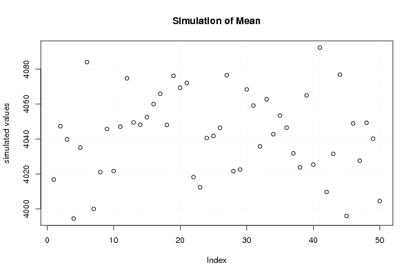
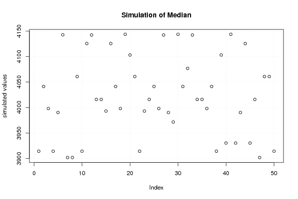
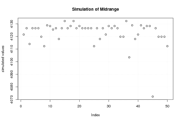
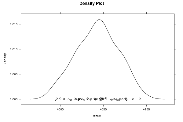
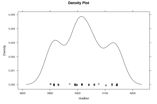
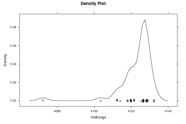
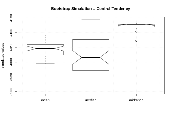
| Title produced by software | Bootstrap Plot - Central Tendency | ||||||||||||||||||||||||||||||||||||||||||||||||||||||||||||||||||||||||||||||||
| Date of computation | Thu, 14 May 2009 12:33:11 -0600 | ||||||||||||||||||||||||||||||||||||||||||||||||||||||||||||||||||||||||||||||||
| Cite this page as follows | Statistical Computations at FreeStatistics.org, Office for Research Development and Education, URL https://freestatistics.org/blog/index.php?v=date/2009/May/14/t12423260143j0c61fbpni6kkw.htm/, Retrieved Thu, 03 Jul 2025 06:49:45 +0000 | ||||||||||||||||||||||||||||||||||||||||||||||||||||||||||||||||||||||||||||||||
| Statistical Computations at FreeStatistics.org, Office for Research Development and Education, URL https://freestatistics.org/blog/index.php?pk=40084, Retrieved Thu, 03 Jul 2025 06:49:45 +0000 | |||||||||||||||||||||||||||||||||||||||||||||||||||||||||||||||||||||||||||||||||
| QR Codes: | |||||||||||||||||||||||||||||||||||||||||||||||||||||||||||||||||||||||||||||||||
|
| |||||||||||||||||||||||||||||||||||||||||||||||||||||||||||||||||||||||||||||||||
| Original text written by user: | |||||||||||||||||||||||||||||||||||||||||||||||||||||||||||||||||||||||||||||||||
| IsPrivate? | No (this computation is public) | ||||||||||||||||||||||||||||||||||||||||||||||||||||||||||||||||||||||||||||||||
| User-defined keywords | |||||||||||||||||||||||||||||||||||||||||||||||||||||||||||||||||||||||||||||||||
| Estimated Impact | 195 | ||||||||||||||||||||||||||||||||||||||||||||||||||||||||||||||||||||||||||||||||
Tree of Dependent Computations | |||||||||||||||||||||||||||||||||||||||||||||||||||||||||||||||||||||||||||||||||
| Family? (F = Feedback message, R = changed R code, M = changed R Module, P = changed Parameters, D = changed Data) | |||||||||||||||||||||||||||||||||||||||||||||||||||||||||||||||||||||||||||||||||
| - [Mean Plot] [] [2009-05-07 16:38:34] [595bbfb6ab1e20d51262e8b831f4c453] - RMPD [(Partial) Autocorrelation Function] [] [2009-05-14 18:27:23] [96b01d8cb0304fe86f721affdc70b94f] - RMP [Bootstrap Plot - Central Tendency] [] [2009-05-14 18:33:11] [5ece983fa688b54e830000b964b580e8] [Current] - [Bootstrap Plot - Central Tendency] [] [2009-05-14 18:35:30] [96b01d8cb0304fe86f721affdc70b94f] - [Bootstrap Plot - Central Tendency] [] [2009-05-14 18:37:18] [96b01d8cb0304fe86f721affdc70b94f] - RMPD [Blocked Bootstrap Plot - Central Tendency] [] [2009-05-14 18:44:53] [96b01d8cb0304fe86f721affdc70b94f] - PD [Blocked Bootstrap Plot - Central Tendency] [] [2009-05-14 18:47:09] [96b01d8cb0304fe86f721affdc70b94f] - P [Blocked Bootstrap Plot - Central Tendency] [] [2009-05-14 18:49:15] [96b01d8cb0304fe86f721affdc70b94f] | |||||||||||||||||||||||||||||||||||||||||||||||||||||||||||||||||||||||||||||||||
| Feedback Forum | |||||||||||||||||||||||||||||||||||||||||||||||||||||||||||||||||||||||||||||||||
Post a new message | |||||||||||||||||||||||||||||||||||||||||||||||||||||||||||||||||||||||||||||||||
Dataset | |||||||||||||||||||||||||||||||||||||||||||||||||||||||||||||||||||||||||||||||||
| Dataseries X: | |||||||||||||||||||||||||||||||||||||||||||||||||||||||||||||||||||||||||||||||||
3851.3 3851.8 3854.1 3858.4 3861.6 3856.3 3855.8 3860.4 3855.1 3839.5 3833 3833.6 3826.8 3818.2 3811.4 3806.8 3810.3 3818.2 3858.9 3867.8 3872.3 3873.3 3876.7 3882.6 3883.5 3882.2 3888.1 3893.7 3901.9 3914.3 3930.3 3948.3 3971.5 3990.1 3993 3998 4015.8 4041.2 4060.7 4076.7 4103 4125.3 4139.7 4146.7 4158 4155.1 4144.8 4148.2 4142.5 4142.1 4145.4 4146.3 4143.5 4149.2 4158.9 4166.1 4179.1 4194.4 4211.7 4226.3 4235.8 4243.6 4258.7 4278.2 4298 4315.1 4334.3 4356 4374 4395.5 4417.8 4432.8 4446.3 | |||||||||||||||||||||||||||||||||||||||||||||||||||||||||||||||||||||||||||||||||
Tables (Output of Computation) | |||||||||||||||||||||||||||||||||||||||||||||||||||||||||||||||||||||||||||||||||
| |||||||||||||||||||||||||||||||||||||||||||||||||||||||||||||||||||||||||||||||||
Figures (Output of Computation) | |||||||||||||||||||||||||||||||||||||||||||||||||||||||||||||||||||||||||||||||||
Input Parameters & R Code | |||||||||||||||||||||||||||||||||||||||||||||||||||||||||||||||||||||||||||||||||
| Parameters (Session): | |||||||||||||||||||||||||||||||||||||||||||||||||||||||||||||||||||||||||||||||||
| par1 = 50 ; | |||||||||||||||||||||||||||||||||||||||||||||||||||||||||||||||||||||||||||||||||
| Parameters (R input): | |||||||||||||||||||||||||||||||||||||||||||||||||||||||||||||||||||||||||||||||||
| par1 = 50 ; | |||||||||||||||||||||||||||||||||||||||||||||||||||||||||||||||||||||||||||||||||
| R code (references can be found in the software module): | |||||||||||||||||||||||||||||||||||||||||||||||||||||||||||||||||||||||||||||||||
par1 <- as.numeric(par1) | |||||||||||||||||||||||||||||||||||||||||||||||||||||||||||||||||||||||||||||||||