Repository of Reproducible Computations

Free Statistics

of Irreproducible Research!

Author's title

Author

*Unverified author*

R Software Module

rwasp_autocorrelation.wasp

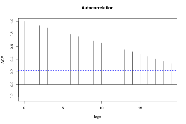
Title produced by software

(Partial) Autocorrelation Function

Date of computation

Thu, 14 May 2009 05:55:18 -0600

Cite this page as follows

Statistical Computations at FreeStatistics.org, Office for Research Development and Education, URL https://freestatistics.org/blog/index.php?v=date/2009/May/14/t12423022163xajjvtqylfowvo.htm/, Retrieved Mon, 29 Apr 2024 03:20:26 +0000

Statistical Computations at FreeStatistics.org, Office for Research Development and Education, URL https://freestatistics.org/blog/index.php?pk=39985, Retrieved Mon, 29 Apr 2024 03:20:26 +0000

QR Codes:

Paste this QR Code to cite your computation.

Original text written by user:

IsPrivate?

No (this computation is public)

User-defined keywords

Estimated Impact

110

Family? (F = Feedback message, R = changed R code, M = changed R Module, P = changed Parameters, D = changed Data)

-       [(Partial) Autocorrelation Function] [Opgave 6bis Oefen...] [2009-05-14 11:55:18] [c0b80eb26a0ae341c828c46b0228b15b] [Current]

Feedback Forum

Post a new message

Dataseries X:

Download CSV

Histogram

Boxplots

5,29
5,29
5,29
5,31
5,33
5,34
5,34
5,37
5,41
5,41
5,38
5,44
5,44
5,46
5,46
5,45
5,46
5,46
5,48
5,47
5,48
5,51
5,55
5,58
5,59
5,6
5,6
5,67
5,71
5,7
5,73
5,72
5,75
5,75
5,77
5,83
5,85
5,87
5,86
5,87
5,93
5,97
5,98
5,99
5,99
6,03
6,06
6,07
6,08
6,08
6,1
6,13
6,14
6,14
6,16
6,2
6,19
6,32
6,32
6,33
6,32
6,33
6,38
6,42
6,46
6,47
6,42
6,48
6,47
6,49
6,48
6,51
6,51
6,52
6,57
6,59
6,62
6,63
6,61
6,64

Summary of computational transaction
Raw Input	view raw input (R code)
Raw Output	view raw output of R engine
Computing time	1 seconds
R Server	'George Udny Yule' @ 72.249.76.132

\begin{tabular}{lllllllll}
\hline
Summary of computational transaction \tabularnewline
Raw Input & view raw input (R code)  \tabularnewline
Raw Output & view raw output of R engine  \tabularnewline
Computing time & 1 seconds \tabularnewline
R Server & 'George Udny Yule' @ 72.249.76.132 \tabularnewline
\hline
\end{tabular}
%Source: https://freestatistics.org/blog/index.php?pk=39985&T=0

[TABLE]
[ROW][C]Summary of computational transaction[/C][/ROW]
[ROW][C]Raw Input[/C][C]view raw input (R code) [/C][/ROW]
[ROW][C]Raw Output[/C][C]view raw output of R engine [/C][/ROW]
[ROW][C]Computing time[/C][C]1 seconds[/C][/ROW]
[ROW][C]R Server[/C][C]'George Udny Yule' @ 72.249.76.132[/C][/ROW]
[/TABLE]
Source: https://freestatistics.org/blog/index.php?pk=39985&T=0

Globally Unique Identifier (entire table): ba.freestatistics.org/blog/index.php?pk=39985&T=0

As an alternative you can also use a QR Code:

The GUIDs for individual cells are displayed in the table below:

Summary of computational transaction
Raw Input	view raw input (R code)
Raw Output	view raw output of R engine
Computing time	1 seconds
R Server	'George Udny Yule' @ 72.249.76.132

Autocorrelation Function
Time lag k	ACF(k)	T-STAT	P-value
1	0.966338	8.6432	0
2	0.933258	8.3473	0
3	0.89778	8.03	0
4	0.862666	7.7159	0
5	0.828653	7.4117	0
6	0.793696	7.099	0
7	0.759581	6.7939	0
8	0.725541	6.4894	0
9	0.692141	6.1907	0
10	0.659391	5.8978	0
11	0.622813	5.5706	0
12	0.588885	5.2671	1e-06
13	0.552433	4.9411	2e-06
14	0.518637	4.6388	7e-06
15	0.480724	4.2997	2.4e-05
16	0.441904	3.9525	8.3e-05
17	0.403959	3.6131	0.000263
18	0.365933	3.273	0.000786
19	0.329968	2.9513	0.002075

\begin{tabular}{lllllllll}
\hline
Autocorrelation Function \tabularnewline
Time lag k & ACF(k) & T-STAT & P-value \tabularnewline
1 & 0.966338 & 8.6432 & 0 \tabularnewline
2 & 0.933258 & 8.3473 & 0 \tabularnewline
3 & 0.89778 & 8.03 & 0 \tabularnewline
4 & 0.862666 & 7.7159 & 0 \tabularnewline
5 & 0.828653 & 7.4117 & 0 \tabularnewline
6 & 0.793696 & 7.099 & 0 \tabularnewline
7 & 0.759581 & 6.7939 & 0 \tabularnewline
8 & 0.725541 & 6.4894 & 0 \tabularnewline
9 & 0.692141 & 6.1907 & 0 \tabularnewline
10 & 0.659391 & 5.8978 & 0 \tabularnewline
11 & 0.622813 & 5.5706 & 0 \tabularnewline
12 & 0.588885 & 5.2671 & 1e-06 \tabularnewline
13 & 0.552433 & 4.9411 & 2e-06 \tabularnewline
14 & 0.518637 & 4.6388 & 7e-06 \tabularnewline
15 & 0.480724 & 4.2997 & 2.4e-05 \tabularnewline
16 & 0.441904 & 3.9525 & 8.3e-05 \tabularnewline
17 & 0.403959 & 3.6131 & 0.000263 \tabularnewline
18 & 0.365933 & 3.273 & 0.000786 \tabularnewline
19 & 0.329968 & 2.9513 & 0.002075 \tabularnewline
\hline
\end{tabular}
%Source: https://freestatistics.org/blog/index.php?pk=39985&T=1

[TABLE]
[ROW][C]Autocorrelation Function[/C][/ROW]
[ROW][C]Time lag k[/C][C]ACF(k)[/C][C]T-STAT[/C][C]P-value[/C][/ROW]
[ROW][C]1[/C][C]0.966338[/C][C]8.6432[/C][C]0[/C][/ROW]
[ROW][C]2[/C][C]0.933258[/C][C]8.3473[/C][C]0[/C][/ROW]
[ROW][C]3[/C][C]0.89778[/C][C]8.03[/C][C]0[/C][/ROW]
[ROW][C]4[/C][C]0.862666[/C][C]7.7159[/C][C]0[/C][/ROW]
[ROW][C]5[/C][C]0.828653[/C][C]7.4117[/C][C]0[/C][/ROW]
[ROW][C]6[/C][C]0.793696[/C][C]7.099[/C][C]0[/C][/ROW]
[ROW][C]7[/C][C]0.759581[/C][C]6.7939[/C][C]0[/C][/ROW]
[ROW][C]8[/C][C]0.725541[/C][C]6.4894[/C][C]0[/C][/ROW]
[ROW][C]9[/C][C]0.692141[/C][C]6.1907[/C][C]0[/C][/ROW]
[ROW][C]10[/C][C]0.659391[/C][C]5.8978[/C][C]0[/C][/ROW]
[ROW][C]11[/C][C]0.622813[/C][C]5.5706[/C][C]0[/C][/ROW]
[ROW][C]12[/C][C]0.588885[/C][C]5.2671[/C][C]1e-06[/C][/ROW]
[ROW][C]13[/C][C]0.552433[/C][C]4.9411[/C][C]2e-06[/C][/ROW]
[ROW][C]14[/C][C]0.518637[/C][C]4.6388[/C][C]7e-06[/C][/ROW]
[ROW][C]15[/C][C]0.480724[/C][C]4.2997[/C][C]2.4e-05[/C][/ROW]
[ROW][C]16[/C][C]0.441904[/C][C]3.9525[/C][C]8.3e-05[/C][/ROW]
[ROW][C]17[/C][C]0.403959[/C][C]3.6131[/C][C]0.000263[/C][/ROW]
[ROW][C]18[/C][C]0.365933[/C][C]3.273[/C][C]0.000786[/C][/ROW]
[ROW][C]19[/C][C]0.329968[/C][C]2.9513[/C][C]0.002075[/C][/ROW]
[/TABLE]
Source: https://freestatistics.org/blog/index.php?pk=39985&T=1

Globally Unique Identifier (entire table): ba.freestatistics.org/blog/index.php?pk=39985&T=1

As an alternative you can also use a QR Code:

The GUIDs for individual cells are displayed in the table below:

Autocorrelation Function
Time lag k	ACF(k)	T-STAT	P-value
1	0.966338	8.6432	0
2	0.933258	8.3473	0
3	0.89778	8.03	0
4	0.862666	7.7159	0
5	0.828653	7.4117	0
6	0.793696	7.099	0
7	0.759581	6.7939	0
8	0.725541	6.4894	0
9	0.692141	6.1907	0
10	0.659391	5.8978	0
11	0.622813	5.5706	0
12	0.588885	5.2671	1e-06
13	0.552433	4.9411	2e-06
14	0.518637	4.6388	7e-06
15	0.480724	4.2997	2.4e-05
16	0.441904	3.9525	8.3e-05
17	0.403959	3.6131	0.000263
18	0.365933	3.273	0.000786
19	0.329968	2.9513	0.002075

Partial Autocorrelation Function
Time lag k	PACF(k)	T-STAT	P-value
1	0.966338	8.6432	0
2	-0.008319	-0.0744	0.470437
3	-0.053272	-0.4765	0.317516
4	-0.013813	-0.1235	0.450991
5	-0.000837	-0.0075	0.497024
6	-0.032957	-0.2948	0.384465
7	-0.008164	-0.073	0.470988
8	-0.016868	-0.1509	0.440228
9	-0.010686	-0.0956	0.462048
10	-0.010196	-0.0912	0.463783
11	-0.077771	-0.6956	0.244346
12	0.016062	0.1437	0.443065
13	-0.054743	-0.4896	0.312867
14	0.013488	0.1206	0.452138
15	-0.084055	-0.7518	0.227187
16	-0.039931	-0.3572	0.36096
17	-0.012715	-0.1137	0.45487
18	-0.02483	-0.2221	0.412405
19	-0.001828	-0.0163	0.493499

\begin{tabular}{lllllllll}
\hline
Partial Autocorrelation Function \tabularnewline
Time lag k & PACF(k) & T-STAT & P-value \tabularnewline
1 & 0.966338 & 8.6432 & 0 \tabularnewline
2 & -0.008319 & -0.0744 & 0.470437 \tabularnewline
3 & -0.053272 & -0.4765 & 0.317516 \tabularnewline
4 & -0.013813 & -0.1235 & 0.450991 \tabularnewline
5 & -0.000837 & -0.0075 & 0.497024 \tabularnewline
6 & -0.032957 & -0.2948 & 0.384465 \tabularnewline
7 & -0.008164 & -0.073 & 0.470988 \tabularnewline
8 & -0.016868 & -0.1509 & 0.440228 \tabularnewline
9 & -0.010686 & -0.0956 & 0.462048 \tabularnewline
10 & -0.010196 & -0.0912 & 0.463783 \tabularnewline
11 & -0.077771 & -0.6956 & 0.244346 \tabularnewline
12 & 0.016062 & 0.1437 & 0.443065 \tabularnewline
13 & -0.054743 & -0.4896 & 0.312867 \tabularnewline
14 & 0.013488 & 0.1206 & 0.452138 \tabularnewline
15 & -0.084055 & -0.7518 & 0.227187 \tabularnewline
16 & -0.039931 & -0.3572 & 0.36096 \tabularnewline
17 & -0.012715 & -0.1137 & 0.45487 \tabularnewline
18 & -0.02483 & -0.2221 & 0.412405 \tabularnewline
19 & -0.001828 & -0.0163 & 0.493499 \tabularnewline
\hline
\end{tabular}
%Source: https://freestatistics.org/blog/index.php?pk=39985&T=2

[TABLE]
[ROW][C]Partial Autocorrelation Function[/C][/ROW]
[ROW][C]Time lag k[/C][C]PACF(k)[/C][C]T-STAT[/C][C]P-value[/C][/ROW]
[ROW][C]1[/C][C]0.966338[/C][C]8.6432[/C][C]0[/C][/ROW]
[ROW][C]2[/C][C]-0.008319[/C][C]-0.0744[/C][C]0.470437[/C][/ROW]
[ROW][C]3[/C][C]-0.053272[/C][C]-0.4765[/C][C]0.317516[/C][/ROW]
[ROW][C]4[/C][C]-0.013813[/C][C]-0.1235[/C][C]0.450991[/C][/ROW]
[ROW][C]5[/C][C]-0.000837[/C][C]-0.0075[/C][C]0.497024[/C][/ROW]
[ROW][C]6[/C][C]-0.032957[/C][C]-0.2948[/C][C]0.384465[/C][/ROW]
[ROW][C]7[/C][C]-0.008164[/C][C]-0.073[/C][C]0.470988[/C][/ROW]
[ROW][C]8[/C][C]-0.016868[/C][C]-0.1509[/C][C]0.440228[/C][/ROW]
[ROW][C]9[/C][C]-0.010686[/C][C]-0.0956[/C][C]0.462048[/C][/ROW]
[ROW][C]10[/C][C]-0.010196[/C][C]-0.0912[/C][C]0.463783[/C][/ROW]
[ROW][C]11[/C][C]-0.077771[/C][C]-0.6956[/C][C]0.244346[/C][/ROW]
[ROW][C]12[/C][C]0.016062[/C][C]0.1437[/C][C]0.443065[/C][/ROW]
[ROW][C]13[/C][C]-0.054743[/C][C]-0.4896[/C][C]0.312867[/C][/ROW]
[ROW][C]14[/C][C]0.013488[/C][C]0.1206[/C][C]0.452138[/C][/ROW]
[ROW][C]15[/C][C]-0.084055[/C][C]-0.7518[/C][C]0.227187[/C][/ROW]
[ROW][C]16[/C][C]-0.039931[/C][C]-0.3572[/C][C]0.36096[/C][/ROW]
[ROW][C]17[/C][C]-0.012715[/C][C]-0.1137[/C][C]0.45487[/C][/ROW]
[ROW][C]18[/C][C]-0.02483[/C][C]-0.2221[/C][C]0.412405[/C][/ROW]
[ROW][C]19[/C][C]-0.001828[/C][C]-0.0163[/C][C]0.493499[/C][/ROW]
[/TABLE]
Source: https://freestatistics.org/blog/index.php?pk=39985&T=2

Globally Unique Identifier (entire table): ba.freestatistics.org/blog/index.php?pk=39985&T=2

As an alternative you can also use a QR Code:

The GUIDs for individual cells are displayed in the table below:

Partial Autocorrelation Function
Time lag k	PACF(k)	T-STAT	P-value
1	0.966338	8.6432	0
2	-0.008319	-0.0744	0.470437
3	-0.053272	-0.4765	0.317516
4	-0.013813	-0.1235	0.450991
5	-0.000837	-0.0075	0.497024
6	-0.032957	-0.2948	0.384465
7	-0.008164	-0.073	0.470988
8	-0.016868	-0.1509	0.440228
9	-0.010686	-0.0956	0.462048
10	-0.010196	-0.0912	0.463783
11	-0.077771	-0.6956	0.244346
12	0.016062	0.1437	0.443065
13	-0.054743	-0.4896	0.312867
14	0.013488	0.1206	0.452138
15	-0.084055	-0.7518	0.227187
16	-0.039931	-0.3572	0.36096
17	-0.012715	-0.1137	0.45487
18	-0.02483	-0.2221	0.412405
19	-0.001828	-0.0163	0.493499

Figure 1

PNG link

Postscript link

PDF link

Figure 2

PNG link

Postscript link

PDF link

Parameters (Session):

par1 = Default ; par2 = 1 ; par3 = 0 ; par4 = 0 ; par5 = 12 ;

Parameters (R input):

par1 = Default ; par2 = 1 ; par3 = 0 ; par4 = 0 ; par5 = 12 ;

R code (references can be found in the software module):

if (par1 == 'Default') {
par1 = 10*log10(length(x))
} else {
par1 <- as.numeric(par1)
}
par2 <- as.numeric(par2)
par3 <- as.numeric(par3)
par4 <- as.numeric(par4)
par5 <- as.numeric(par5)
if (par2 == 0) {
x <- log(x)
} else {
x <- (x ^ par2 - 1) / par2
}
if (par3 > 0) x <- diff(x,lag=1,difference=par3)
if (par4 > 0) x <- diff(x,lag=par5,difference=par4)
bitmap(file='pic1.png')
racf <- acf(x,par1,main='Autocorrelation',xlab='lags',ylab='ACF')
dev.off()
bitmap(file='pic2.png')
rpacf <- pacf(x,par1,main='Partial Autocorrelation',xlab='lags',ylab='PACF')
dev.off()
(myacf <- c(racf$acf))
(mypacf <- c(rpacf$acf))
lengthx <- length(x)
sqrtn <- sqrt(lengthx)
load(file='createtable')
a<-table.start()
a<-table.row.start(a)
a<-table.element(a,'Autocorrelation Function',4,TRUE)
a<-table.row.end(a)
a<-table.row.start(a)
a<-table.element(a,'Time lag k',header=TRUE)
a<-table.element(a,hyperlink('basics.htm','ACF(k)','click here for more information about the Autocorrelation Function'),header=TRUE)
a<-table.element(a,'T-STAT',header=TRUE)
a<-table.element(a,'P-value',header=TRUE)
a<-table.row.end(a)
for (i in 2:(par1+1)) {
a<-table.row.start(a)
a<-table.element(a,i-1,header=TRUE)
a<-table.element(a,round(myacf[i],6))
mytstat <- myacf[i]*sqrtn
a<-table.element(a,round(mytstat,4))
a<-table.element(a,round(1-pt(abs(mytstat),lengthx),6))
a<-table.row.end(a)
}
a<-table.end(a)
table.save(a,file='mytable.tab')
a<-table.start()
a<-table.row.start(a)
a<-table.element(a,'Partial Autocorrelation Function',4,TRUE)
a<-table.row.end(a)
a<-table.row.start(a)
a<-table.element(a,'Time lag k',header=TRUE)
a<-table.element(a,hyperlink('basics.htm','PACF(k)','click here for more information about the Partial Autocorrelation Function'),header=TRUE)
a<-table.element(a,'T-STAT',header=TRUE)
a<-table.element(a,'P-value',header=TRUE)
a<-table.row.end(a)
for (i in 1:par1) {
a<-table.row.start(a)
a<-table.element(a,i,header=TRUE)
a<-table.element(a,round(mypacf[i],6))
mytstat <- mypacf[i]*sqrtn
a<-table.element(a,round(mytstat,4))
a<-table.element(a,round(1-pt(abs(mytstat),lengthx),6))
a<-table.row.end(a)
}
a<-table.end(a)
table.save(a,file='mytable1.tab')

Free Statistics

Description of Statistical Computation

Tree of Dependent Computations

Dataset

Tables (Output of Computation)

Figures (Output of Computation)

Input Parameters & R Code