Free Statistics

of Irreproducible Research!

Author's title

Time Series Analysis (new) - autocorrelation - gemiddelde prijs strip - Del...

Author

*Unverified author*

R Software Module

rwasp_autocorrelation.wasp

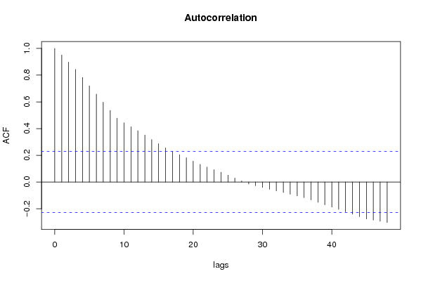
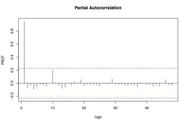
Title produced by software

(Partial) Autocorrelation Function

Date of computation

Thu, 14 May 2009 02:38:46 -0600

Cite this page as follows

Statistical Computations at FreeStatistics.org, Office for Research Development and Education, URL https://freestatistics.org/blog/index.php?v=date/2009/May/14/t1242290513fgoqjpli4h67jbe.htm/, Retrieved Sun, 28 Apr 2024 19:59:45 +0000

Statistical Computations at FreeStatistics.org, Office for Research Development and Education, URL https://freestatistics.org/blog/index.php?pk=39942, Retrieved Sun, 28 Apr 2024 19:59:45 +0000

QR Codes:

Paste this QR Code to cite your computation.

Original text written by user:

IsPrivate?

No (this computation is public)

User-defined keywords

Estimated Impact

187

Family? (F = Feedback message, R = changed R code, M = changed R Module, P = changed Parameters, D = changed Data)

-     [(Partial) Autocorrelation Function] [] [2008-12-16 08:41:39] [a18c43c8b63fa6800a53bb187b9ddd45]
-   PD    [(Partial) Autocorrelation Function] [Time Series Analy...] [2009-05-14 08:38:46] [2c54c43cc67b7c768ab8b58e4cb451d8] [Current]
-   PD      [(Partial) Autocorrelation Function] [Time Series Analy...] [2009-05-14 08:43:55] [40e8bd42426f0e7582df61f417649af3] 

Feedback Forum

Post a new message

Dataseries X:

Download CSV

Histogram

Boxplots

5,11
5,11
5,11
5,1
5,1
5,1
5,1
5,1
5,12
5,25
5,26
5,26
5,26
5,26
5,26
5,26
5,29
5,3
5,33
5,33
5,35
5,38
5,38
5,38
5,38
5,38
5,39
5,39
5,4
5,4
5,4
5,4
5,4
5,41
5,41
5,41
5,41
5,41
5,42
5,42
5,42
5,42
5,43
5,43
5,45
5,51
5,51
5,51
5,51
5,51
5,51
5,53
5,53
5,53
5,53
5,52
5,53
5,54
5,54
5,57
5,56
5,57
5,58
5,61
5,66
5,68
5,69
5,7
5,72
5,71
5,69
5,7
5,7

Summary of computational transaction
Raw Input	view raw input (R code)
Raw Output	view raw output of R engine
Computing time	1 seconds
R Server	'George Udny Yule' @ 72.249.76.132

\begin{tabular}{lllllllll}
\hline
Summary of computational transaction \tabularnewline
Raw Input & view raw input (R code)  \tabularnewline
Raw Output & view raw output of R engine  \tabularnewline
Computing time & 1 seconds \tabularnewline
R Server & 'George Udny Yule' @ 72.249.76.132 \tabularnewline
\hline
\end{tabular}
%Source: https://freestatistics.org/blog/index.php?pk=39942&T=0

[TABLE]
[ROW][C]Summary of computational transaction[/C][/ROW]
[ROW][C]Raw Input[/C][C]view raw input (R code) [/C][/ROW]
[ROW][C]Raw Output[/C][C]view raw output of R engine [/C][/ROW]
[ROW][C]Computing time[/C][C]1 seconds[/C][/ROW]
[ROW][C]R Server[/C][C]'George Udny Yule' @ 72.249.76.132[/C][/ROW]
[/TABLE]
Source: https://freestatistics.org/blog/index.php?pk=39942&T=0

Globally Unique Identifier (entire table): ba.freestatistics.org/blog/index.php?pk=39942&T=0

As an alternative you can also use a QR Code:

The GUIDs for individual cells are displayed in the table below:

Summary of computational transaction
Raw Input	view raw input (R code)
Raw Output	view raw output of R engine
Computing time	1 seconds
R Server	'George Udny Yule' @ 72.249.76.132

Autocorrelation Function
Time lag k	ACF(k)	T-STAT	P-value
1	0.950666	8.1225	0
2	0.896984	7.6638	0
3	0.842689	7.1999	0
4	0.782461	6.6853	0
5	0.719835	6.1503	0
6	0.658468	5.626	0
7	0.598066	5.1099	1e-06
8	0.536048	4.58	9e-06
9	0.477852	4.0828	5.6e-05
10	0.443287	3.7874	0.000155
11	0.413709	3.5347	0.000356
12	0.383901	3.28	0.000796
13	0.351951	3.0071	0.001808
14	0.318033	2.7173	0.004108
15	0.287055	2.4526	0.008286
16	0.255791	2.1855	0.016031
17	0.229813	1.9635	0.026697
18	0.204887	1.7506	0.042112
19	0.181886	1.554	0.062251
20	0.156352	1.3359	0.09287
21	0.13233	1.1306	0.130956
22	0.111771	0.955	0.171372
23	0.09314	0.7958	0.214368
24	0.073267	0.626	0.266637
25	0.05153	0.4403	0.330521
26	0.029506	0.2521	0.400835
27	0.007952	0.0679	0.473008
28	-0.014605	-0.1248	0.450517
29	-0.028281	-0.2416	0.404872
30	-0.040888	-0.3493	0.363917
31	-0.054116	-0.4624	0.322595
32	-0.066572	-0.5688	0.285622
33	-0.079027	-0.6752	0.250838
34	-0.091205	-0.7793	0.219175
35	-0.103573	-0.8849	0.189551
36	-0.116697	-0.9971	0.161014
37	-0.134217	-1.1468	0.127614
38	-0.152407	-1.3022	0.098477
39	-0.169983	-1.4523	0.075346
40	-0.187846	-1.605	0.05641
41	-0.204745	-1.7493	0.042217
42	-0.222457	-1.9007	0.030647
43	-0.240177	-2.0521	0.021875
44	-0.259617	-2.2182	0.014827
45	-0.276828	-2.3652	0.010339
46	-0.284812	-2.4334	0.008702
47	-0.293465	-2.5074	0.007194
48	-0.302684	-2.5861	0.00585

\begin{tabular}{lllllllll}
\hline
Autocorrelation Function \tabularnewline
Time lag k & ACF(k) & T-STAT & P-value \tabularnewline
1 & 0.950666 & 8.1225 & 0 \tabularnewline
2 & 0.896984 & 7.6638 & 0 \tabularnewline
3 & 0.842689 & 7.1999 & 0 \tabularnewline
4 & 0.782461 & 6.6853 & 0 \tabularnewline
5 & 0.719835 & 6.1503 & 0 \tabularnewline
6 & 0.658468 & 5.626 & 0 \tabularnewline
7 & 0.598066 & 5.1099 & 1e-06 \tabularnewline
8 & 0.536048 & 4.58 & 9e-06 \tabularnewline
9 & 0.477852 & 4.0828 & 5.6e-05 \tabularnewline
10 & 0.443287 & 3.7874 & 0.000155 \tabularnewline
11 & 0.413709 & 3.5347 & 0.000356 \tabularnewline
12 & 0.383901 & 3.28 & 0.000796 \tabularnewline
13 & 0.351951 & 3.0071 & 0.001808 \tabularnewline
14 & 0.318033 & 2.7173 & 0.004108 \tabularnewline
15 & 0.287055 & 2.4526 & 0.008286 \tabularnewline
16 & 0.255791 & 2.1855 & 0.016031 \tabularnewline
17 & 0.229813 & 1.9635 & 0.026697 \tabularnewline
18 & 0.204887 & 1.7506 & 0.042112 \tabularnewline
19 & 0.181886 & 1.554 & 0.062251 \tabularnewline
20 & 0.156352 & 1.3359 & 0.09287 \tabularnewline
21 & 0.13233 & 1.1306 & 0.130956 \tabularnewline
22 & 0.111771 & 0.955 & 0.171372 \tabularnewline
23 & 0.09314 & 0.7958 & 0.214368 \tabularnewline
24 & 0.073267 & 0.626 & 0.266637 \tabularnewline
25 & 0.05153 & 0.4403 & 0.330521 \tabularnewline
26 & 0.029506 & 0.2521 & 0.400835 \tabularnewline
27 & 0.007952 & 0.0679 & 0.473008 \tabularnewline
28 & -0.014605 & -0.1248 & 0.450517 \tabularnewline
29 & -0.028281 & -0.2416 & 0.404872 \tabularnewline
30 & -0.040888 & -0.3493 & 0.363917 \tabularnewline
31 & -0.054116 & -0.4624 & 0.322595 \tabularnewline
32 & -0.066572 & -0.5688 & 0.285622 \tabularnewline
33 & -0.079027 & -0.6752 & 0.250838 \tabularnewline
34 & -0.091205 & -0.7793 & 0.219175 \tabularnewline
35 & -0.103573 & -0.8849 & 0.189551 \tabularnewline
36 & -0.116697 & -0.9971 & 0.161014 \tabularnewline
37 & -0.134217 & -1.1468 & 0.127614 \tabularnewline
38 & -0.152407 & -1.3022 & 0.098477 \tabularnewline
39 & -0.169983 & -1.4523 & 0.075346 \tabularnewline
40 & -0.187846 & -1.605 & 0.05641 \tabularnewline
41 & -0.204745 & -1.7493 & 0.042217 \tabularnewline
42 & -0.222457 & -1.9007 & 0.030647 \tabularnewline
43 & -0.240177 & -2.0521 & 0.021875 \tabularnewline
44 & -0.259617 & -2.2182 & 0.014827 \tabularnewline
45 & -0.276828 & -2.3652 & 0.010339 \tabularnewline
46 & -0.284812 & -2.4334 & 0.008702 \tabularnewline
47 & -0.293465 & -2.5074 & 0.007194 \tabularnewline
48 & -0.302684 & -2.5861 & 0.00585 \tabularnewline
\hline
\end{tabular}
%Source: https://freestatistics.org/blog/index.php?pk=39942&T=1

[TABLE]
[ROW][C]Autocorrelation Function[/C][/ROW]
[ROW][C]Time lag k[/C][C]ACF(k)[/C][C]T-STAT[/C][C]P-value[/C][/ROW]
[ROW][C]1[/C][C]0.950666[/C][C]8.1225[/C][C]0[/C][/ROW]
[ROW][C]2[/C][C]0.896984[/C][C]7.6638[/C][C]0[/C][/ROW]
[ROW][C]3[/C][C]0.842689[/C][C]7.1999[/C][C]0[/C][/ROW]
[ROW][C]4[/C][C]0.782461[/C][C]6.6853[/C][C]0[/C][/ROW]
[ROW][C]5[/C][C]0.719835[/C][C]6.1503[/C][C]0[/C][/ROW]
[ROW][C]6[/C][C]0.658468[/C][C]5.626[/C][C]0[/C][/ROW]
[ROW][C]7[/C][C]0.598066[/C][C]5.1099[/C][C]1e-06[/C][/ROW]
[ROW][C]8[/C][C]0.536048[/C][C]4.58[/C][C]9e-06[/C][/ROW]
[ROW][C]9[/C][C]0.477852[/C][C]4.0828[/C][C]5.6e-05[/C][/ROW]
[ROW][C]10[/C][C]0.443287[/C][C]3.7874[/C][C]0.000155[/C][/ROW]
[ROW][C]11[/C][C]0.413709[/C][C]3.5347[/C][C]0.000356[/C][/ROW]
[ROW][C]12[/C][C]0.383901[/C][C]3.28[/C][C]0.000796[/C][/ROW]
[ROW][C]13[/C][C]0.351951[/C][C]3.0071[/C][C]0.001808[/C][/ROW]
[ROW][C]14[/C][C]0.318033[/C][C]2.7173[/C][C]0.004108[/C][/ROW]
[ROW][C]15[/C][C]0.287055[/C][C]2.4526[/C][C]0.008286[/C][/ROW]
[ROW][C]16[/C][C]0.255791[/C][C]2.1855[/C][C]0.016031[/C][/ROW]
[ROW][C]17[/C][C]0.229813[/C][C]1.9635[/C][C]0.026697[/C][/ROW]
[ROW][C]18[/C][C]0.204887[/C][C]1.7506[/C][C]0.042112[/C][/ROW]
[ROW][C]19[/C][C]0.181886[/C][C]1.554[/C][C]0.062251[/C][/ROW]
[ROW][C]20[/C][C]0.156352[/C][C]1.3359[/C][C]0.09287[/C][/ROW]
[ROW][C]21[/C][C]0.13233[/C][C]1.1306[/C][C]0.130956[/C][/ROW]
[ROW][C]22[/C][C]0.111771[/C][C]0.955[/C][C]0.171372[/C][/ROW]
[ROW][C]23[/C][C]0.09314[/C][C]0.7958[/C][C]0.214368[/C][/ROW]
[ROW][C]24[/C][C]0.073267[/C][C]0.626[/C][C]0.266637[/C][/ROW]
[ROW][C]25[/C][C]0.05153[/C][C]0.4403[/C][C]0.330521[/C][/ROW]
[ROW][C]26[/C][C]0.029506[/C][C]0.2521[/C][C]0.400835[/C][/ROW]
[ROW][C]27[/C][C]0.007952[/C][C]0.0679[/C][C]0.473008[/C][/ROW]
[ROW][C]28[/C][C]-0.014605[/C][C]-0.1248[/C][C]0.450517[/C][/ROW]
[ROW][C]29[/C][C]-0.028281[/C][C]-0.2416[/C][C]0.404872[/C][/ROW]
[ROW][C]30[/C][C]-0.040888[/C][C]-0.3493[/C][C]0.363917[/C][/ROW]
[ROW][C]31[/C][C]-0.054116[/C][C]-0.4624[/C][C]0.322595[/C][/ROW]
[ROW][C]32[/C][C]-0.066572[/C][C]-0.5688[/C][C]0.285622[/C][/ROW]
[ROW][C]33[/C][C]-0.079027[/C][C]-0.6752[/C][C]0.250838[/C][/ROW]
[ROW][C]34[/C][C]-0.091205[/C][C]-0.7793[/C][C]0.219175[/C][/ROW]
[ROW][C]35[/C][C]-0.103573[/C][C]-0.8849[/C][C]0.189551[/C][/ROW]
[ROW][C]36[/C][C]-0.116697[/C][C]-0.9971[/C][C]0.161014[/C][/ROW]
[ROW][C]37[/C][C]-0.134217[/C][C]-1.1468[/C][C]0.127614[/C][/ROW]
[ROW][C]38[/C][C]-0.152407[/C][C]-1.3022[/C][C]0.098477[/C][/ROW]
[ROW][C]39[/C][C]-0.169983[/C][C]-1.4523[/C][C]0.075346[/C][/ROW]
[ROW][C]40[/C][C]-0.187846[/C][C]-1.605[/C][C]0.05641[/C][/ROW]
[ROW][C]41[/C][C]-0.204745[/C][C]-1.7493[/C][C]0.042217[/C][/ROW]
[ROW][C]42[/C][C]-0.222457[/C][C]-1.9007[/C][C]0.030647[/C][/ROW]
[ROW][C]43[/C][C]-0.240177[/C][C]-2.0521[/C][C]0.021875[/C][/ROW]
[ROW][C]44[/C][C]-0.259617[/C][C]-2.2182[/C][C]0.014827[/C][/ROW]
[ROW][C]45[/C][C]-0.276828[/C][C]-2.3652[/C][C]0.010339[/C][/ROW]
[ROW][C]46[/C][C]-0.284812[/C][C]-2.4334[/C][C]0.008702[/C][/ROW]
[ROW][C]47[/C][C]-0.293465[/C][C]-2.5074[/C][C]0.007194[/C][/ROW]
[ROW][C]48[/C][C]-0.302684[/C][C]-2.5861[/C][C]0.00585[/C][/ROW]
[/TABLE]
Source: https://freestatistics.org/blog/index.php?pk=39942&T=1

Globally Unique Identifier (entire table): ba.freestatistics.org/blog/index.php?pk=39942&T=1

As an alternative you can also use a QR Code:

The GUIDs for individual cells are displayed in the table below:

Autocorrelation Function
Time lag k	ACF(k)	T-STAT	P-value
1	0.950666	8.1225	0
2	0.896984	7.6638	0
3	0.842689	7.1999	0
4	0.782461	6.6853	0
5	0.719835	6.1503	0
6	0.658468	5.626	0
7	0.598066	5.1099	1e-06
8	0.536048	4.58	9e-06
9	0.477852	4.0828	5.6e-05
10	0.443287	3.7874	0.000155
11	0.413709	3.5347	0.000356
12	0.383901	3.28	0.000796
13	0.351951	3.0071	0.001808
14	0.318033	2.7173	0.004108
15	0.287055	2.4526	0.008286
16	0.255791	2.1855	0.016031
17	0.229813	1.9635	0.026697
18	0.204887	1.7506	0.042112
19	0.181886	1.554	0.062251
20	0.156352	1.3359	0.09287
21	0.13233	1.1306	0.130956
22	0.111771	0.955	0.171372
23	0.09314	0.7958	0.214368
24	0.073267	0.626	0.266637
25	0.05153	0.4403	0.330521
26	0.029506	0.2521	0.400835
27	0.007952	0.0679	0.473008
28	-0.014605	-0.1248	0.450517
29	-0.028281	-0.2416	0.404872
30	-0.040888	-0.3493	0.363917
31	-0.054116	-0.4624	0.322595
32	-0.066572	-0.5688	0.285622
33	-0.079027	-0.6752	0.250838
34	-0.091205	-0.7793	0.219175
35	-0.103573	-0.8849	0.189551
36	-0.116697	-0.9971	0.161014
37	-0.134217	-1.1468	0.127614
38	-0.152407	-1.3022	0.098477
39	-0.169983	-1.4523	0.075346
40	-0.187846	-1.605	0.05641
41	-0.204745	-1.7493	0.042217
42	-0.222457	-1.9007	0.030647
43	-0.240177	-2.0521	0.021875
44	-0.259617	-2.2182	0.014827
45	-0.276828	-2.3652	0.010339
46	-0.284812	-2.4334	0.008702
47	-0.293465	-2.5074	0.007194
48	-0.302684	-2.5861	0.00585

Partial Autocorrelation Function
Time lag k	PACF(k)	T-STAT	P-value
1	0.950666	8.1225	0
2	-0.070473	-0.6021	0.274479
3	-0.032804	-0.2803	0.390028
4	-0.091051	-0.7779	0.219559
5	-0.054186	-0.463	0.322382
6	-0.021303	-0.182	0.428039
7	-0.024465	-0.209	0.417503
8	-0.053232	-0.4548	0.325297
9	0.000172	0.0015	0.499417
10	0.206542	1.7647	0.040899
11	0.011961	0.1022	0.459442
12	-0.03555	-0.3037	0.381094
13	-0.080726	-0.6897	0.246278
14	-0.063692	-0.5442	0.293988
15	0.009077	0.0776	0.469199
16	-0.026661	-0.2278	0.410221
17	0.026078	0.2228	0.412151
18	-0.007488	-0.064	0.474581
19	0.055631	0.4753	0.317993
20	-0.038564	-0.3295	0.371363
21	-0.017046	-0.1456	0.442303
22	-0.018421	-0.1574	0.437688
23	-0.021282	-0.1818	0.42811
24	-0.026935	-0.2301	0.409316
25	-0.044502	-0.3802	0.352442
26	-0.003166	-0.0271	0.489246
27	-0.006092	-0.0521	0.479315
28	-0.012278	-0.1049	0.458372
29	0.063328	0.5411	0.295052
30	-0.017914	-0.1531	0.439389
31	-0.018542	-0.1584	0.43728
32	-0.0214	-0.1828	0.427714
33	-0.029601	-0.2529	0.400525
34	-0.033984	-0.2904	0.386182
35	-0.020476	-0.1749	0.430802
36	-0.028302	-0.2418	0.4048
37	-0.062113	-0.5307	0.298621
38	0.01532	0.1309	0.448109
39	-0.006071	-0.0519	0.479387
40	-0.022688	-0.1938	0.423418
41	-0.022221	-0.1899	0.424976
42	-0.051512	-0.4401	0.330576
43	-0.026985	-0.2306	0.409152
44	-0.052842	-0.4515	0.326489
45	-0.002938	-0.0251	0.490021
46	0.053723	0.459	0.323797
47	-0.020738	-0.1772	0.429926
48	-0.027479	-0.2348	0.407518

\begin{tabular}{lllllllll}
\hline
Partial Autocorrelation Function \tabularnewline
Time lag k & PACF(k) & T-STAT & P-value \tabularnewline
1 & 0.950666 & 8.1225 & 0 \tabularnewline
2 & -0.070473 & -0.6021 & 0.274479 \tabularnewline
3 & -0.032804 & -0.2803 & 0.390028 \tabularnewline
4 & -0.091051 & -0.7779 & 0.219559 \tabularnewline
5 & -0.054186 & -0.463 & 0.322382 \tabularnewline
6 & -0.021303 & -0.182 & 0.428039 \tabularnewline
7 & -0.024465 & -0.209 & 0.417503 \tabularnewline
8 & -0.053232 & -0.4548 & 0.325297 \tabularnewline
9 & 0.000172 & 0.0015 & 0.499417 \tabularnewline
10 & 0.206542 & 1.7647 & 0.040899 \tabularnewline
11 & 0.011961 & 0.1022 & 0.459442 \tabularnewline
12 & -0.03555 & -0.3037 & 0.381094 \tabularnewline
13 & -0.080726 & -0.6897 & 0.246278 \tabularnewline
14 & -0.063692 & -0.5442 & 0.293988 \tabularnewline
15 & 0.009077 & 0.0776 & 0.469199 \tabularnewline
16 & -0.026661 & -0.2278 & 0.410221 \tabularnewline
17 & 0.026078 & 0.2228 & 0.412151 \tabularnewline
18 & -0.007488 & -0.064 & 0.474581 \tabularnewline
19 & 0.055631 & 0.4753 & 0.317993 \tabularnewline
20 & -0.038564 & -0.3295 & 0.371363 \tabularnewline
21 & -0.017046 & -0.1456 & 0.442303 \tabularnewline
22 & -0.018421 & -0.1574 & 0.437688 \tabularnewline
23 & -0.021282 & -0.1818 & 0.42811 \tabularnewline
24 & -0.026935 & -0.2301 & 0.409316 \tabularnewline
25 & -0.044502 & -0.3802 & 0.352442 \tabularnewline
26 & -0.003166 & -0.0271 & 0.489246 \tabularnewline
27 & -0.006092 & -0.0521 & 0.479315 \tabularnewline
28 & -0.012278 & -0.1049 & 0.458372 \tabularnewline
29 & 0.063328 & 0.5411 & 0.295052 \tabularnewline
30 & -0.017914 & -0.1531 & 0.439389 \tabularnewline
31 & -0.018542 & -0.1584 & 0.43728 \tabularnewline
32 & -0.0214 & -0.1828 & 0.427714 \tabularnewline
33 & -0.029601 & -0.2529 & 0.400525 \tabularnewline
34 & -0.033984 & -0.2904 & 0.386182 \tabularnewline
35 & -0.020476 & -0.1749 & 0.430802 \tabularnewline
36 & -0.028302 & -0.2418 & 0.4048 \tabularnewline
37 & -0.062113 & -0.5307 & 0.298621 \tabularnewline
38 & 0.01532 & 0.1309 & 0.448109 \tabularnewline
39 & -0.006071 & -0.0519 & 0.479387 \tabularnewline
40 & -0.022688 & -0.1938 & 0.423418 \tabularnewline
41 & -0.022221 & -0.1899 & 0.424976 \tabularnewline
42 & -0.051512 & -0.4401 & 0.330576 \tabularnewline
43 & -0.026985 & -0.2306 & 0.409152 \tabularnewline
44 & -0.052842 & -0.4515 & 0.326489 \tabularnewline
45 & -0.002938 & -0.0251 & 0.490021 \tabularnewline
46 & 0.053723 & 0.459 & 0.323797 \tabularnewline
47 & -0.020738 & -0.1772 & 0.429926 \tabularnewline
48 & -0.027479 & -0.2348 & 0.407518 \tabularnewline
\hline
\end{tabular}
%Source: https://freestatistics.org/blog/index.php?pk=39942&T=2

[TABLE]
[ROW][C]Partial Autocorrelation Function[/C][/ROW]
[ROW][C]Time lag k[/C][C]PACF(k)[/C][C]T-STAT[/C][C]P-value[/C][/ROW]
[ROW][C]1[/C][C]0.950666[/C][C]8.1225[/C][C]0[/C][/ROW]
[ROW][C]2[/C][C]-0.070473[/C][C]-0.6021[/C][C]0.274479[/C][/ROW]
[ROW][C]3[/C][C]-0.032804[/C][C]-0.2803[/C][C]0.390028[/C][/ROW]
[ROW][C]4[/C][C]-0.091051[/C][C]-0.7779[/C][C]0.219559[/C][/ROW]
[ROW][C]5[/C][C]-0.054186[/C][C]-0.463[/C][C]0.322382[/C][/ROW]
[ROW][C]6[/C][C]-0.021303[/C][C]-0.182[/C][C]0.428039[/C][/ROW]
[ROW][C]7[/C][C]-0.024465[/C][C]-0.209[/C][C]0.417503[/C][/ROW]
[ROW][C]8[/C][C]-0.053232[/C][C]-0.4548[/C][C]0.325297[/C][/ROW]
[ROW][C]9[/C][C]0.000172[/C][C]0.0015[/C][C]0.499417[/C][/ROW]
[ROW][C]10[/C][C]0.206542[/C][C]1.7647[/C][C]0.040899[/C][/ROW]
[ROW][C]11[/C][C]0.011961[/C][C]0.1022[/C][C]0.459442[/C][/ROW]
[ROW][C]12[/C][C]-0.03555[/C][C]-0.3037[/C][C]0.381094[/C][/ROW]
[ROW][C]13[/C][C]-0.080726[/C][C]-0.6897[/C][C]0.246278[/C][/ROW]
[ROW][C]14[/C][C]-0.063692[/C][C]-0.5442[/C][C]0.293988[/C][/ROW]
[ROW][C]15[/C][C]0.009077[/C][C]0.0776[/C][C]0.469199[/C][/ROW]
[ROW][C]16[/C][C]-0.026661[/C][C]-0.2278[/C][C]0.410221[/C][/ROW]
[ROW][C]17[/C][C]0.026078[/C][C]0.2228[/C][C]0.412151[/C][/ROW]
[ROW][C]18[/C][C]-0.007488[/C][C]-0.064[/C][C]0.474581[/C][/ROW]
[ROW][C]19[/C][C]0.055631[/C][C]0.4753[/C][C]0.317993[/C][/ROW]
[ROW][C]20[/C][C]-0.038564[/C][C]-0.3295[/C][C]0.371363[/C][/ROW]
[ROW][C]21[/C][C]-0.017046[/C][C]-0.1456[/C][C]0.442303[/C][/ROW]
[ROW][C]22[/C][C]-0.018421[/C][C]-0.1574[/C][C]0.437688[/C][/ROW]
[ROW][C]23[/C][C]-0.021282[/C][C]-0.1818[/C][C]0.42811[/C][/ROW]
[ROW][C]24[/C][C]-0.026935[/C][C]-0.2301[/C][C]0.409316[/C][/ROW]
[ROW][C]25[/C][C]-0.044502[/C][C]-0.3802[/C][C]0.352442[/C][/ROW]
[ROW][C]26[/C][C]-0.003166[/C][C]-0.0271[/C][C]0.489246[/C][/ROW]
[ROW][C]27[/C][C]-0.006092[/C][C]-0.0521[/C][C]0.479315[/C][/ROW]
[ROW][C]28[/C][C]-0.012278[/C][C]-0.1049[/C][C]0.458372[/C][/ROW]
[ROW][C]29[/C][C]0.063328[/C][C]0.5411[/C][C]0.295052[/C][/ROW]
[ROW][C]30[/C][C]-0.017914[/C][C]-0.1531[/C][C]0.439389[/C][/ROW]
[ROW][C]31[/C][C]-0.018542[/C][C]-0.1584[/C][C]0.43728[/C][/ROW]
[ROW][C]32[/C][C]-0.0214[/C][C]-0.1828[/C][C]0.427714[/C][/ROW]
[ROW][C]33[/C][C]-0.029601[/C][C]-0.2529[/C][C]0.400525[/C][/ROW]
[ROW][C]34[/C][C]-0.033984[/C][C]-0.2904[/C][C]0.386182[/C][/ROW]
[ROW][C]35[/C][C]-0.020476[/C][C]-0.1749[/C][C]0.430802[/C][/ROW]
[ROW][C]36[/C][C]-0.028302[/C][C]-0.2418[/C][C]0.4048[/C][/ROW]
[ROW][C]37[/C][C]-0.062113[/C][C]-0.5307[/C][C]0.298621[/C][/ROW]
[ROW][C]38[/C][C]0.01532[/C][C]0.1309[/C][C]0.448109[/C][/ROW]
[ROW][C]39[/C][C]-0.006071[/C][C]-0.0519[/C][C]0.479387[/C][/ROW]
[ROW][C]40[/C][C]-0.022688[/C][C]-0.1938[/C][C]0.423418[/C][/ROW]
[ROW][C]41[/C][C]-0.022221[/C][C]-0.1899[/C][C]0.424976[/C][/ROW]
[ROW][C]42[/C][C]-0.051512[/C][C]-0.4401[/C][C]0.330576[/C][/ROW]
[ROW][C]43[/C][C]-0.026985[/C][C]-0.2306[/C][C]0.409152[/C][/ROW]
[ROW][C]44[/C][C]-0.052842[/C][C]-0.4515[/C][C]0.326489[/C][/ROW]
[ROW][C]45[/C][C]-0.002938[/C][C]-0.0251[/C][C]0.490021[/C][/ROW]
[ROW][C]46[/C][C]0.053723[/C][C]0.459[/C][C]0.323797[/C][/ROW]
[ROW][C]47[/C][C]-0.020738[/C][C]-0.1772[/C][C]0.429926[/C][/ROW]
[ROW][C]48[/C][C]-0.027479[/C][C]-0.2348[/C][C]0.407518[/C][/ROW]
[/TABLE]
Source: https://freestatistics.org/blog/index.php?pk=39942&T=2

Globally Unique Identifier (entire table): ba.freestatistics.org/blog/index.php?pk=39942&T=2

As an alternative you can also use a QR Code:

The GUIDs for individual cells are displayed in the table below:

Partial Autocorrelation Function
Time lag k	PACF(k)	T-STAT	P-value
1	0.950666	8.1225	0
2	-0.070473	-0.6021	0.274479
3	-0.032804	-0.2803	0.390028
4	-0.091051	-0.7779	0.219559
5	-0.054186	-0.463	0.322382
6	-0.021303	-0.182	0.428039
7	-0.024465	-0.209	0.417503
8	-0.053232	-0.4548	0.325297
9	0.000172	0.0015	0.499417
10	0.206542	1.7647	0.040899
11	0.011961	0.1022	0.459442
12	-0.03555	-0.3037	0.381094
13	-0.080726	-0.6897	0.246278
14	-0.063692	-0.5442	0.293988
15	0.009077	0.0776	0.469199
16	-0.026661	-0.2278	0.410221
17	0.026078	0.2228	0.412151
18	-0.007488	-0.064	0.474581
19	0.055631	0.4753	0.317993
20	-0.038564	-0.3295	0.371363
21	-0.017046	-0.1456	0.442303
22	-0.018421	-0.1574	0.437688
23	-0.021282	-0.1818	0.42811
24	-0.026935	-0.2301	0.409316
25	-0.044502	-0.3802	0.352442
26	-0.003166	-0.0271	0.489246
27	-0.006092	-0.0521	0.479315
28	-0.012278	-0.1049	0.458372
29	0.063328	0.5411	0.295052
30	-0.017914	-0.1531	0.439389
31	-0.018542	-0.1584	0.43728
32	-0.0214	-0.1828	0.427714
33	-0.029601	-0.2529	0.400525
34	-0.033984	-0.2904	0.386182
35	-0.020476	-0.1749	0.430802
36	-0.028302	-0.2418	0.4048
37	-0.062113	-0.5307	0.298621
38	0.01532	0.1309	0.448109
39	-0.006071	-0.0519	0.479387
40	-0.022688	-0.1938	0.423418
41	-0.022221	-0.1899	0.424976
42	-0.051512	-0.4401	0.330576
43	-0.026985	-0.2306	0.409152
44	-0.052842	-0.4515	0.326489
45	-0.002938	-0.0251	0.490021
46	0.053723	0.459	0.323797
47	-0.020738	-0.1772	0.429926
48	-0.027479	-0.2348	0.407518

Figure 1

PNG link

Postscript link

PDF link

Figure 2

PNG link

Postscript link

PDF link

Parameters (Session):

par1 = 48 ; par2 = 1 ; par3 = 0 ; par4 = 0 ; par5 = 12 ;

Parameters (R input):

par1 = 48 ; par2 = 1 ; par3 = 0 ; par4 = 0 ; par5 = 12 ;

R code (references can be found in the software module):

if (par1 == 'Default') {
par1 = 10*log10(length(x))
} else {
par1 <- as.numeric(par1)
}
par2 <- as.numeric(par2)
par3 <- as.numeric(par3)
par4 <- as.numeric(par4)
par5 <- as.numeric(par5)
if (par2 == 0) {
x <- log(x)
} else {
x <- (x ^ par2 - 1) / par2
}
if (par3 > 0) x <- diff(x,lag=1,difference=par3)
if (par4 > 0) x <- diff(x,lag=par5,difference=par4)
bitmap(file='pic1.png')
racf <- acf(x,par1,main='Autocorrelation',xlab='lags',ylab='ACF')
dev.off()
bitmap(file='pic2.png')
rpacf <- pacf(x,par1,main='Partial Autocorrelation',xlab='lags',ylab='PACF')
dev.off()
(myacf <- c(racf$acf))
(mypacf <- c(rpacf$acf))
lengthx <- length(x)
sqrtn <- sqrt(lengthx)
load(file='createtable')
a<-table.start()
a<-table.row.start(a)
a<-table.element(a,'Autocorrelation Function',4,TRUE)
a<-table.row.end(a)
a<-table.row.start(a)
a<-table.element(a,'Time lag k',header=TRUE)
a<-table.element(a,hyperlink('basics.htm','ACF(k)','click here for more information about the Autocorrelation Function'),header=TRUE)
a<-table.element(a,'T-STAT',header=TRUE)
a<-table.element(a,'P-value',header=TRUE)
a<-table.row.end(a)
for (i in 2:(par1+1)) {
a<-table.row.start(a)
a<-table.element(a,i-1,header=TRUE)
a<-table.element(a,round(myacf[i],6))
mytstat <- myacf[i]*sqrtn
a<-table.element(a,round(mytstat,4))
a<-table.element(a,round(1-pt(abs(mytstat),lengthx),6))
a<-table.row.end(a)
}
a<-table.end(a)
table.save(a,file='mytable.tab')
a<-table.start()
a<-table.row.start(a)
a<-table.element(a,'Partial Autocorrelation Function',4,TRUE)
a<-table.row.end(a)
a<-table.row.start(a)
a<-table.element(a,'Time lag k',header=TRUE)
a<-table.element(a,hyperlink('basics.htm','PACF(k)','click here for more information about the Partial Autocorrelation Function'),header=TRUE)
a<-table.element(a,'T-STAT',header=TRUE)
a<-table.element(a,'P-value',header=TRUE)
a<-table.row.end(a)
for (i in 1:par1) {
a<-table.row.start(a)
a<-table.element(a,i,header=TRUE)
a<-table.element(a,round(mypacf[i],6))
mytstat <- mypacf[i]*sqrtn
a<-table.element(a,round(mytstat,4))
a<-table.element(a,round(1-pt(abs(mytstat),lengthx),6))
a<-table.row.end(a)
}
a<-table.end(a)
table.save(a,file='mytable1.tab')

Free Statistics

Description of Statistical Computation

Time Series Analysis (new) - autocorrelation - gemiddelde prijs strip - Del...

Tree of Dependent Computations

Dataset

Tables (Output of Computation)

Figures (Output of Computation)

Input Parameters & R Code