Free Statistics

of Irreproducible Research!

Author's title

Opgave 6bis Oefening 2 - Autocorrelatiefunctie - Wisselkoers Euro in Dollar...

Author

*Unverified author*

R Software Module

rwasp_autocorrelation.wasp

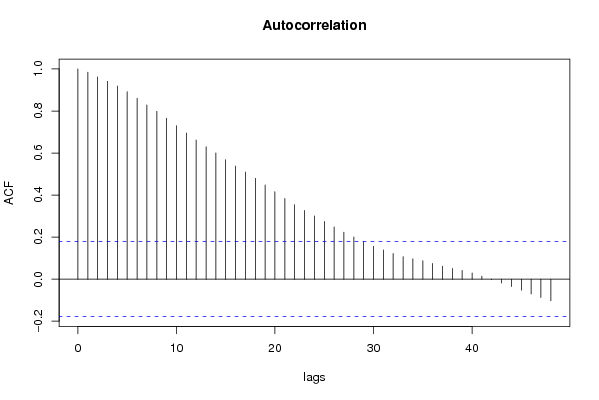
Title produced by software

(Partial) Autocorrelation Function

Date of computation

Wed, 13 May 2009 10:16:39 -0600

Cite this page as follows

Statistical Computations at FreeStatistics.org, Office for Research Development and Education, URL https://freestatistics.org/blog/index.php?v=date/2009/May/13/t1242231476njkn0xg6c7l25ob.htm/, Retrieved Wed, 08 May 2024 05:23:23 +0000

Statistical Computations at FreeStatistics.org, Office for Research Development and Education, URL https://freestatistics.org/blog/index.php?pk=39865, Retrieved Wed, 08 May 2024 05:23:23 +0000

QR Codes:

Paste this QR Code to cite your computation.

Original text written by user:

IsPrivate?

No (this computation is public)

User-defined keywords

Estimated Impact

132

Family? (F = Feedback message, R = changed R code, M = changed R Module, P = changed Parameters, D = changed Data)

-       [(Partial) Autocorrelation Function] [Opgave 6bis Oefen...] [2009-05-13 16:16:39] [69a8397eb9368d6355c6053ed100f2c7] [Current]

Feedback Forum

Post a new message

Dataseries X:

Download CSV

Histogram

Boxplots

Summary of computational transaction
Raw Input	view raw input (R code)
Raw Output	view raw output of R engine
Computing time	2 seconds
R Server	'Sir Ronald Aylmer Fisher' @ 193.190.124.24

\begin{tabular}{lllllllll}
\hline
Summary of computational transaction \tabularnewline
Raw Input & view raw input (R code)  \tabularnewline
Raw Output & view raw output of R engine  \tabularnewline
Computing time & 2 seconds \tabularnewline
R Server & 'Sir Ronald Aylmer Fisher' @ 193.190.124.24 \tabularnewline
\hline
\end{tabular}
%Source: https://freestatistics.org/blog/index.php?pk=39865&T=0

[TABLE]
[ROW][C]Summary of computational transaction[/C][/ROW]
[ROW][C]Raw Input[/C][C]view raw input (R code) [/C][/ROW]
[ROW][C]Raw Output[/C][C]view raw output of R engine [/C][/ROW]
[ROW][C]Computing time[/C][C]2 seconds[/C][/ROW]
[ROW][C]R Server[/C][C]'Sir Ronald Aylmer Fisher' @ 193.190.124.24[/C][/ROW]
[/TABLE]
Source: https://freestatistics.org/blog/index.php?pk=39865&T=0

Globally Unique Identifier (entire table): ba.freestatistics.org/blog/index.php?pk=39865&T=0

As an alternative you can also use a QR Code:

The GUIDs for individual cells are displayed in the table below:

Summary of computational transaction
Raw Input	view raw input (R code)
Raw Output	view raw output of R engine
Computing time	2 seconds
R Server	'Sir Ronald Aylmer Fisher' @ 193.190.124.24

Autocorrelation Function
Time lag k	ACF(k)	T-STAT	P-value
1	0.984862	10.8335	0
2	0.961785	10.5796	0
3	0.941009	10.3511	0
4	0.918558	10.1041	0
5	0.891452	9.806	0
6	0.860702	9.4677	0
7	0.828327	9.1116	0
8	0.798218	8.7804	0
9	0.765902	8.4249	0
10	0.730152	8.0317	0
11	0.694831	7.6431	0
12	0.661703	7.2787	0
13	0.630107	6.9312	0
14	0.600038	6.6004	0
15	0.568551	6.2541	0
16	0.538044	5.9185	0
17	0.509533	5.6049	0
18	0.479725	5.277	0
19	0.447797	4.9258	1e-06
20	0.415608	4.5717	6e-06
21	0.384152	4.2257	2.3e-05
22	0.35456	3.9002	7.9e-05
23	0.32676	3.5944	0.000236
24	0.300817	3.309	0.000617
25	0.274344	3.0178	0.001553
26	0.248131	2.7294	0.003645
27	0.223719	2.4609	0.007635
28	0.20096	2.2106	0.014473
29	0.17818	1.96	0.026149
30	0.157024	1.7273	0.043336
31	0.139343	1.5328	0.063971
32	0.122343	1.3458	0.090446
33	0.107174	1.1789	0.120374
34	0.096704	1.0637	0.144782
35	0.087537	0.9629	0.168758
36	0.075094	0.826	0.205206
37	0.061374	0.6751	0.250445
38	0.05088	0.5597	0.288366
39	0.041412	0.4555	0.324773
40	0.029861	0.3285	0.371564
41	0.0139	0.1529	0.439365
42	-0.002211	-0.0243	0.490317
43	-0.018134	-0.1995	0.421113
44	-0.035241	-0.3877	0.349477
45	-0.052197	-0.5742	0.28346
46	-0.070007	-0.7701	0.221378
47	-0.087478	-0.9623	0.16892
48	-0.102798	-1.1308	0.130192

\begin{tabular}{lllllllll}
\hline
Autocorrelation Function \tabularnewline
Time lag k & ACF(k) & T-STAT & P-value \tabularnewline
1 & 0.984862 & 10.8335 & 0 \tabularnewline
2 & 0.961785 & 10.5796 & 0 \tabularnewline
3 & 0.941009 & 10.3511 & 0 \tabularnewline
4 & 0.918558 & 10.1041 & 0 \tabularnewline
5 & 0.891452 & 9.806 & 0 \tabularnewline
6 & 0.860702 & 9.4677 & 0 \tabularnewline
7 & 0.828327 & 9.1116 & 0 \tabularnewline
8 & 0.798218 & 8.7804 & 0 \tabularnewline
9 & 0.765902 & 8.4249 & 0 \tabularnewline
10 & 0.730152 & 8.0317 & 0 \tabularnewline
11 & 0.694831 & 7.6431 & 0 \tabularnewline
12 & 0.661703 & 7.2787 & 0 \tabularnewline
13 & 0.630107 & 6.9312 & 0 \tabularnewline
14 & 0.600038 & 6.6004 & 0 \tabularnewline
15 & 0.568551 & 6.2541 & 0 \tabularnewline
16 & 0.538044 & 5.9185 & 0 \tabularnewline
17 & 0.509533 & 5.6049 & 0 \tabularnewline
18 & 0.479725 & 5.277 & 0 \tabularnewline
19 & 0.447797 & 4.9258 & 1e-06 \tabularnewline
20 & 0.415608 & 4.5717 & 6e-06 \tabularnewline
21 & 0.384152 & 4.2257 & 2.3e-05 \tabularnewline
22 & 0.35456 & 3.9002 & 7.9e-05 \tabularnewline
23 & 0.32676 & 3.5944 & 0.000236 \tabularnewline
24 & 0.300817 & 3.309 & 0.000617 \tabularnewline
25 & 0.274344 & 3.0178 & 0.001553 \tabularnewline
26 & 0.248131 & 2.7294 & 0.003645 \tabularnewline
27 & 0.223719 & 2.4609 & 0.007635 \tabularnewline
28 & 0.20096 & 2.2106 & 0.014473 \tabularnewline
29 & 0.17818 & 1.96 & 0.026149 \tabularnewline
30 & 0.157024 & 1.7273 & 0.043336 \tabularnewline
31 & 0.139343 & 1.5328 & 0.063971 \tabularnewline
32 & 0.122343 & 1.3458 & 0.090446 \tabularnewline
33 & 0.107174 & 1.1789 & 0.120374 \tabularnewline
34 & 0.096704 & 1.0637 & 0.144782 \tabularnewline
35 & 0.087537 & 0.9629 & 0.168758 \tabularnewline
36 & 0.075094 & 0.826 & 0.205206 \tabularnewline
37 & 0.061374 & 0.6751 & 0.250445 \tabularnewline
38 & 0.05088 & 0.5597 & 0.288366 \tabularnewline
39 & 0.041412 & 0.4555 & 0.324773 \tabularnewline
40 & 0.029861 & 0.3285 & 0.371564 \tabularnewline
41 & 0.0139 & 0.1529 & 0.439365 \tabularnewline
42 & -0.002211 & -0.0243 & 0.490317 \tabularnewline
43 & -0.018134 & -0.1995 & 0.421113 \tabularnewline
44 & -0.035241 & -0.3877 & 0.349477 \tabularnewline
45 & -0.052197 & -0.5742 & 0.28346 \tabularnewline
46 & -0.070007 & -0.7701 & 0.221378 \tabularnewline
47 & -0.087478 & -0.9623 & 0.16892 \tabularnewline
48 & -0.102798 & -1.1308 & 0.130192 \tabularnewline
\hline
\end{tabular}
%Source: https://freestatistics.org/blog/index.php?pk=39865&T=1

[TABLE]
[ROW][C]Autocorrelation Function[/C][/ROW]
[ROW][C]Time lag k[/C][C]ACF(k)[/C][C]T-STAT[/C][C]P-value[/C][/ROW]
[ROW][C]1[/C][C]0.984862[/C][C]10.8335[/C][C]0[/C][/ROW]
[ROW][C]2[/C][C]0.961785[/C][C]10.5796[/C][C]0[/C][/ROW]
[ROW][C]3[/C][C]0.941009[/C][C]10.3511[/C][C]0[/C][/ROW]
[ROW][C]4[/C][C]0.918558[/C][C]10.1041[/C][C]0[/C][/ROW]
[ROW][C]5[/C][C]0.891452[/C][C]9.806[/C][C]0[/C][/ROW]
[ROW][C]6[/C][C]0.860702[/C][C]9.4677[/C][C]0[/C][/ROW]
[ROW][C]7[/C][C]0.828327[/C][C]9.1116[/C][C]0[/C][/ROW]
[ROW][C]8[/C][C]0.798218[/C][C]8.7804[/C][C]0[/C][/ROW]
[ROW][C]9[/C][C]0.765902[/C][C]8.4249[/C][C]0[/C][/ROW]
[ROW][C]10[/C][C]0.730152[/C][C]8.0317[/C][C]0[/C][/ROW]
[ROW][C]11[/C][C]0.694831[/C][C]7.6431[/C][C]0[/C][/ROW]
[ROW][C]12[/C][C]0.661703[/C][C]7.2787[/C][C]0[/C][/ROW]
[ROW][C]13[/C][C]0.630107[/C][C]6.9312[/C][C]0[/C][/ROW]
[ROW][C]14[/C][C]0.600038[/C][C]6.6004[/C][C]0[/C][/ROW]
[ROW][C]15[/C][C]0.568551[/C][C]6.2541[/C][C]0[/C][/ROW]
[ROW][C]16[/C][C]0.538044[/C][C]5.9185[/C][C]0[/C][/ROW]
[ROW][C]17[/C][C]0.509533[/C][C]5.6049[/C][C]0[/C][/ROW]
[ROW][C]18[/C][C]0.479725[/C][C]5.277[/C][C]0[/C][/ROW]
[ROW][C]19[/C][C]0.447797[/C][C]4.9258[/C][C]1e-06[/C][/ROW]
[ROW][C]20[/C][C]0.415608[/C][C]4.5717[/C][C]6e-06[/C][/ROW]
[ROW][C]21[/C][C]0.384152[/C][C]4.2257[/C][C]2.3e-05[/C][/ROW]
[ROW][C]22[/C][C]0.35456[/C][C]3.9002[/C][C]7.9e-05[/C][/ROW]
[ROW][C]23[/C][C]0.32676[/C][C]3.5944[/C][C]0.000236[/C][/ROW]
[ROW][C]24[/C][C]0.300817[/C][C]3.309[/C][C]0.000617[/C][/ROW]
[ROW][C]25[/C][C]0.274344[/C][C]3.0178[/C][C]0.001553[/C][/ROW]
[ROW][C]26[/C][C]0.248131[/C][C]2.7294[/C][C]0.003645[/C][/ROW]
[ROW][C]27[/C][C]0.223719[/C][C]2.4609[/C][C]0.007635[/C][/ROW]
[ROW][C]28[/C][C]0.20096[/C][C]2.2106[/C][C]0.014473[/C][/ROW]
[ROW][C]29[/C][C]0.17818[/C][C]1.96[/C][C]0.026149[/C][/ROW]
[ROW][C]30[/C][C]0.157024[/C][C]1.7273[/C][C]0.043336[/C][/ROW]
[ROW][C]31[/C][C]0.139343[/C][C]1.5328[/C][C]0.063971[/C][/ROW]
[ROW][C]32[/C][C]0.122343[/C][C]1.3458[/C][C]0.090446[/C][/ROW]
[ROW][C]33[/C][C]0.107174[/C][C]1.1789[/C][C]0.120374[/C][/ROW]
[ROW][C]34[/C][C]0.096704[/C][C]1.0637[/C][C]0.144782[/C][/ROW]
[ROW][C]35[/C][C]0.087537[/C][C]0.9629[/C][C]0.168758[/C][/ROW]
[ROW][C]36[/C][C]0.075094[/C][C]0.826[/C][C]0.205206[/C][/ROW]
[ROW][C]37[/C][C]0.061374[/C][C]0.6751[/C][C]0.250445[/C][/ROW]
[ROW][C]38[/C][C]0.05088[/C][C]0.5597[/C][C]0.288366[/C][/ROW]
[ROW][C]39[/C][C]0.041412[/C][C]0.4555[/C][C]0.324773[/C][/ROW]
[ROW][C]40[/C][C]0.029861[/C][C]0.3285[/C][C]0.371564[/C][/ROW]
[ROW][C]41[/C][C]0.0139[/C][C]0.1529[/C][C]0.439365[/C][/ROW]
[ROW][C]42[/C][C]-0.002211[/C][C]-0.0243[/C][C]0.490317[/C][/ROW]
[ROW][C]43[/C][C]-0.018134[/C][C]-0.1995[/C][C]0.421113[/C][/ROW]
[ROW][C]44[/C][C]-0.035241[/C][C]-0.3877[/C][C]0.349477[/C][/ROW]
[ROW][C]45[/C][C]-0.052197[/C][C]-0.5742[/C][C]0.28346[/C][/ROW]
[ROW][C]46[/C][C]-0.070007[/C][C]-0.7701[/C][C]0.221378[/C][/ROW]
[ROW][C]47[/C][C]-0.087478[/C][C]-0.9623[/C][C]0.16892[/C][/ROW]
[ROW][C]48[/C][C]-0.102798[/C][C]-1.1308[/C][C]0.130192[/C][/ROW]
[/TABLE]
Source: https://freestatistics.org/blog/index.php?pk=39865&T=1

Globally Unique Identifier (entire table): ba.freestatistics.org/blog/index.php?pk=39865&T=1

As an alternative you can also use a QR Code:

The GUIDs for individual cells are displayed in the table below:

Autocorrelation Function
Time lag k	ACF(k)	T-STAT	P-value
1	0.984862	10.8335	0
2	0.961785	10.5796	0
3	0.941009	10.3511	0
4	0.918558	10.1041	0
5	0.891452	9.806	0
6	0.860702	9.4677	0
7	0.828327	9.1116	0
8	0.798218	8.7804	0
9	0.765902	8.4249	0
10	0.730152	8.0317	0
11	0.694831	7.6431	0
12	0.661703	7.2787	0
13	0.630107	6.9312	0
14	0.600038	6.6004	0
15	0.568551	6.2541	0
16	0.538044	5.9185	0
17	0.509533	5.6049	0
18	0.479725	5.277	0
19	0.447797	4.9258	1e-06
20	0.415608	4.5717	6e-06
21	0.384152	4.2257	2.3e-05
22	0.35456	3.9002	7.9e-05
23	0.32676	3.5944	0.000236
24	0.300817	3.309	0.000617
25	0.274344	3.0178	0.001553
26	0.248131	2.7294	0.003645
27	0.223719	2.4609	0.007635
28	0.20096	2.2106	0.014473
29	0.17818	1.96	0.026149
30	0.157024	1.7273	0.043336
31	0.139343	1.5328	0.063971
32	0.122343	1.3458	0.090446
33	0.107174	1.1789	0.120374
34	0.096704	1.0637	0.144782
35	0.087537	0.9629	0.168758
36	0.075094	0.826	0.205206
37	0.061374	0.6751	0.250445
38	0.05088	0.5597	0.288366
39	0.041412	0.4555	0.324773
40	0.029861	0.3285	0.371564
41	0.0139	0.1529	0.439365
42	-0.002211	-0.0243	0.490317
43	-0.018134	-0.1995	0.421113
44	-0.035241	-0.3877	0.349477
45	-0.052197	-0.5742	0.28346
46	-0.070007	-0.7701	0.221378
47	-0.087478	-0.9623	0.16892
48	-0.102798	-1.1308	0.130192

Partial Autocorrelation Function
Time lag k	PACF(k)	T-STAT	P-value
1	0.984862	10.8335	0
2	-0.271816	-2.99	0.00169
3	0.144249	1.5867	0.057591
4	-0.142079	-1.5629	0.060347
5	-0.111188	-1.2231	0.11184
6	-0.089869	-0.9886	0.162427
7	-0.048463	-0.5331	0.297472
8	0.08726	0.9599	0.16952
9	-0.141559	-1.5571	0.061023
10	-0.031889	-0.3508	0.363183
11	0.018215	0.2004	0.420766
12	0.019085	0.2099	0.417038
13	0.033595	0.3695	0.356183
14	0.038154	0.4197	0.337727
15	-0.078885	-0.8677	0.193629
16	0.036221	0.3984	0.345508
17	-0.025595	-0.2815	0.389386
18	-0.08081	-0.8889	0.187907
19	-0.052496	-0.5775	0.282351
20	-0.039997	-0.44	0.330373
21	-0.003108	-0.0342	0.486393
22	0.01892	0.2081	0.417741
23	0.04996	0.5496	0.291818
24	0.061281	0.6741	0.250771
25	-0.090563	-0.9962	0.160572
26	0.013134	0.1445	0.442683
27	0.017773	0.1955	0.422663
28	-0.007321	-0.0805	0.467975
29	-0.027621	-0.3038	0.380888
30	0.033058	0.3636	0.35838
31	0.049768	0.5474	0.29254
32	-0.078915	-0.8681	0.193539
33	0.090072	0.9908	0.161881
34	0.114088	1.255	0.105954
35	-0.056023	-0.6163	0.269443
36	-0.140736	-1.5481	0.062105
37	-0.009214	-0.1014	0.459719
38	0.067752	0.7453	0.228777
39	-0.082919	-0.9121	0.181764
40	-0.055613	-0.6117	0.270926
41	-0.138842	-1.5273	0.064652
42	0.019801	0.2178	0.413971
43	-0.08341	-0.9175	0.180352
44	0.019888	0.2188	0.413599
45	0.090212	0.9923	0.161509
46	-0.072102	-0.7931	0.214628
47	0.034334	0.3777	0.353168
48	-0.012424	-0.1367	0.445763

\begin{tabular}{lllllllll}
\hline
Partial Autocorrelation Function \tabularnewline
Time lag k & PACF(k) & T-STAT & P-value \tabularnewline
1 & 0.984862 & 10.8335 & 0 \tabularnewline
2 & -0.271816 & -2.99 & 0.00169 \tabularnewline
3 & 0.144249 & 1.5867 & 0.057591 \tabularnewline
4 & -0.142079 & -1.5629 & 0.060347 \tabularnewline
5 & -0.111188 & -1.2231 & 0.11184 \tabularnewline
6 & -0.089869 & -0.9886 & 0.162427 \tabularnewline
7 & -0.048463 & -0.5331 & 0.297472 \tabularnewline
8 & 0.08726 & 0.9599 & 0.16952 \tabularnewline
9 & -0.141559 & -1.5571 & 0.061023 \tabularnewline
10 & -0.031889 & -0.3508 & 0.363183 \tabularnewline
11 & 0.018215 & 0.2004 & 0.420766 \tabularnewline
12 & 0.019085 & 0.2099 & 0.417038 \tabularnewline
13 & 0.033595 & 0.3695 & 0.356183 \tabularnewline
14 & 0.038154 & 0.4197 & 0.337727 \tabularnewline
15 & -0.078885 & -0.8677 & 0.193629 \tabularnewline
16 & 0.036221 & 0.3984 & 0.345508 \tabularnewline
17 & -0.025595 & -0.2815 & 0.389386 \tabularnewline
18 & -0.08081 & -0.8889 & 0.187907 \tabularnewline
19 & -0.052496 & -0.5775 & 0.282351 \tabularnewline
20 & -0.039997 & -0.44 & 0.330373 \tabularnewline
21 & -0.003108 & -0.0342 & 0.486393 \tabularnewline
22 & 0.01892 & 0.2081 & 0.417741 \tabularnewline
23 & 0.04996 & 0.5496 & 0.291818 \tabularnewline
24 & 0.061281 & 0.6741 & 0.250771 \tabularnewline
25 & -0.090563 & -0.9962 & 0.160572 \tabularnewline
26 & 0.013134 & 0.1445 & 0.442683 \tabularnewline
27 & 0.017773 & 0.1955 & 0.422663 \tabularnewline
28 & -0.007321 & -0.0805 & 0.467975 \tabularnewline
29 & -0.027621 & -0.3038 & 0.380888 \tabularnewline
30 & 0.033058 & 0.3636 & 0.35838 \tabularnewline
31 & 0.049768 & 0.5474 & 0.29254 \tabularnewline
32 & -0.078915 & -0.8681 & 0.193539 \tabularnewline
33 & 0.090072 & 0.9908 & 0.161881 \tabularnewline
34 & 0.114088 & 1.255 & 0.105954 \tabularnewline
35 & -0.056023 & -0.6163 & 0.269443 \tabularnewline
36 & -0.140736 & -1.5481 & 0.062105 \tabularnewline
37 & -0.009214 & -0.1014 & 0.459719 \tabularnewline
38 & 0.067752 & 0.7453 & 0.228777 \tabularnewline
39 & -0.082919 & -0.9121 & 0.181764 \tabularnewline
40 & -0.055613 & -0.6117 & 0.270926 \tabularnewline
41 & -0.138842 & -1.5273 & 0.064652 \tabularnewline
42 & 0.019801 & 0.2178 & 0.413971 \tabularnewline
43 & -0.08341 & -0.9175 & 0.180352 \tabularnewline
44 & 0.019888 & 0.2188 & 0.413599 \tabularnewline
45 & 0.090212 & 0.9923 & 0.161509 \tabularnewline
46 & -0.072102 & -0.7931 & 0.214628 \tabularnewline
47 & 0.034334 & 0.3777 & 0.353168 \tabularnewline
48 & -0.012424 & -0.1367 & 0.445763 \tabularnewline
\hline
\end{tabular}
%Source: https://freestatistics.org/blog/index.php?pk=39865&T=2

[TABLE]
[ROW][C]Partial Autocorrelation Function[/C][/ROW]
[ROW][C]Time lag k[/C][C]PACF(k)[/C][C]T-STAT[/C][C]P-value[/C][/ROW]
[ROW][C]1[/C][C]0.984862[/C][C]10.8335[/C][C]0[/C][/ROW]
[ROW][C]2[/C][C]-0.271816[/C][C]-2.99[/C][C]0.00169[/C][/ROW]
[ROW][C]3[/C][C]0.144249[/C][C]1.5867[/C][C]0.057591[/C][/ROW]
[ROW][C]4[/C][C]-0.142079[/C][C]-1.5629[/C][C]0.060347[/C][/ROW]
[ROW][C]5[/C][C]-0.111188[/C][C]-1.2231[/C][C]0.11184[/C][/ROW]
[ROW][C]6[/C][C]-0.089869[/C][C]-0.9886[/C][C]0.162427[/C][/ROW]
[ROW][C]7[/C][C]-0.048463[/C][C]-0.5331[/C][C]0.297472[/C][/ROW]
[ROW][C]8[/C][C]0.08726[/C][C]0.9599[/C][C]0.16952[/C][/ROW]
[ROW][C]9[/C][C]-0.141559[/C][C]-1.5571[/C][C]0.061023[/C][/ROW]
[ROW][C]10[/C][C]-0.031889[/C][C]-0.3508[/C][C]0.363183[/C][/ROW]
[ROW][C]11[/C][C]0.018215[/C][C]0.2004[/C][C]0.420766[/C][/ROW]
[ROW][C]12[/C][C]0.019085[/C][C]0.2099[/C][C]0.417038[/C][/ROW]
[ROW][C]13[/C][C]0.033595[/C][C]0.3695[/C][C]0.356183[/C][/ROW]
[ROW][C]14[/C][C]0.038154[/C][C]0.4197[/C][C]0.337727[/C][/ROW]
[ROW][C]15[/C][C]-0.078885[/C][C]-0.8677[/C][C]0.193629[/C][/ROW]
[ROW][C]16[/C][C]0.036221[/C][C]0.3984[/C][C]0.345508[/C][/ROW]
[ROW][C]17[/C][C]-0.025595[/C][C]-0.2815[/C][C]0.389386[/C][/ROW]
[ROW][C]18[/C][C]-0.08081[/C][C]-0.8889[/C][C]0.187907[/C][/ROW]
[ROW][C]19[/C][C]-0.052496[/C][C]-0.5775[/C][C]0.282351[/C][/ROW]
[ROW][C]20[/C][C]-0.039997[/C][C]-0.44[/C][C]0.330373[/C][/ROW]
[ROW][C]21[/C][C]-0.003108[/C][C]-0.0342[/C][C]0.486393[/C][/ROW]
[ROW][C]22[/C][C]0.01892[/C][C]0.2081[/C][C]0.417741[/C][/ROW]
[ROW][C]23[/C][C]0.04996[/C][C]0.5496[/C][C]0.291818[/C][/ROW]
[ROW][C]24[/C][C]0.061281[/C][C]0.6741[/C][C]0.250771[/C][/ROW]
[ROW][C]25[/C][C]-0.090563[/C][C]-0.9962[/C][C]0.160572[/C][/ROW]
[ROW][C]26[/C][C]0.013134[/C][C]0.1445[/C][C]0.442683[/C][/ROW]
[ROW][C]27[/C][C]0.017773[/C][C]0.1955[/C][C]0.422663[/C][/ROW]
[ROW][C]28[/C][C]-0.007321[/C][C]-0.0805[/C][C]0.467975[/C][/ROW]
[ROW][C]29[/C][C]-0.027621[/C][C]-0.3038[/C][C]0.380888[/C][/ROW]
[ROW][C]30[/C][C]0.033058[/C][C]0.3636[/C][C]0.35838[/C][/ROW]
[ROW][C]31[/C][C]0.049768[/C][C]0.5474[/C][C]0.29254[/C][/ROW]
[ROW][C]32[/C][C]-0.078915[/C][C]-0.8681[/C][C]0.193539[/C][/ROW]
[ROW][C]33[/C][C]0.090072[/C][C]0.9908[/C][C]0.161881[/C][/ROW]
[ROW][C]34[/C][C]0.114088[/C][C]1.255[/C][C]0.105954[/C][/ROW]
[ROW][C]35[/C][C]-0.056023[/C][C]-0.6163[/C][C]0.269443[/C][/ROW]
[ROW][C]36[/C][C]-0.140736[/C][C]-1.5481[/C][C]0.062105[/C][/ROW]
[ROW][C]37[/C][C]-0.009214[/C][C]-0.1014[/C][C]0.459719[/C][/ROW]
[ROW][C]38[/C][C]0.067752[/C][C]0.7453[/C][C]0.228777[/C][/ROW]
[ROW][C]39[/C][C]-0.082919[/C][C]-0.9121[/C][C]0.181764[/C][/ROW]
[ROW][C]40[/C][C]-0.055613[/C][C]-0.6117[/C][C]0.270926[/C][/ROW]
[ROW][C]41[/C][C]-0.138842[/C][C]-1.5273[/C][C]0.064652[/C][/ROW]
[ROW][C]42[/C][C]0.019801[/C][C]0.2178[/C][C]0.413971[/C][/ROW]
[ROW][C]43[/C][C]-0.08341[/C][C]-0.9175[/C][C]0.180352[/C][/ROW]
[ROW][C]44[/C][C]0.019888[/C][C]0.2188[/C][C]0.413599[/C][/ROW]
[ROW][C]45[/C][C]0.090212[/C][C]0.9923[/C][C]0.161509[/C][/ROW]
[ROW][C]46[/C][C]-0.072102[/C][C]-0.7931[/C][C]0.214628[/C][/ROW]
[ROW][C]47[/C][C]0.034334[/C][C]0.3777[/C][C]0.353168[/C][/ROW]
[ROW][C]48[/C][C]-0.012424[/C][C]-0.1367[/C][C]0.445763[/C][/ROW]
[/TABLE]
Source: https://freestatistics.org/blog/index.php?pk=39865&T=2

Globally Unique Identifier (entire table): ba.freestatistics.org/blog/index.php?pk=39865&T=2

As an alternative you can also use a QR Code:

The GUIDs for individual cells are displayed in the table below:

Partial Autocorrelation Function
Time lag k	PACF(k)	T-STAT	P-value
1	0.984862	10.8335	0
2	-0.271816	-2.99	0.00169
3	0.144249	1.5867	0.057591
4	-0.142079	-1.5629	0.060347
5	-0.111188	-1.2231	0.11184
6	-0.089869	-0.9886	0.162427
7	-0.048463	-0.5331	0.297472
8	0.08726	0.9599	0.16952
9	-0.141559	-1.5571	0.061023
10	-0.031889	-0.3508	0.363183
11	0.018215	0.2004	0.420766
12	0.019085	0.2099	0.417038
13	0.033595	0.3695	0.356183
14	0.038154	0.4197	0.337727
15	-0.078885	-0.8677	0.193629
16	0.036221	0.3984	0.345508
17	-0.025595	-0.2815	0.389386
18	-0.08081	-0.8889	0.187907
19	-0.052496	-0.5775	0.282351
20	-0.039997	-0.44	0.330373
21	-0.003108	-0.0342	0.486393
22	0.01892	0.2081	0.417741
23	0.04996	0.5496	0.291818
24	0.061281	0.6741	0.250771
25	-0.090563	-0.9962	0.160572
26	0.013134	0.1445	0.442683
27	0.017773	0.1955	0.422663
28	-0.007321	-0.0805	0.467975
29	-0.027621	-0.3038	0.380888
30	0.033058	0.3636	0.35838
31	0.049768	0.5474	0.29254
32	-0.078915	-0.8681	0.193539
33	0.090072	0.9908	0.161881
34	0.114088	1.255	0.105954
35	-0.056023	-0.6163	0.269443
36	-0.140736	-1.5481	0.062105
37	-0.009214	-0.1014	0.459719
38	0.067752	0.7453	0.228777
39	-0.082919	-0.9121	0.181764
40	-0.055613	-0.6117	0.270926
41	-0.138842	-1.5273	0.064652
42	0.019801	0.2178	0.413971
43	-0.08341	-0.9175	0.180352
44	0.019888	0.2188	0.413599
45	0.090212	0.9923	0.161509
46	-0.072102	-0.7931	0.214628
47	0.034334	0.3777	0.353168
48	-0.012424	-0.1367	0.445763

Figure 1

PNG link

Postscript link

PDF link

Figure 2

PNG link

Postscript link

PDF link

Parameters (Session):

par1 = 48 ; par2 = 1 ; par3 = 0 ; par4 = 0 ; par5 = 12 ;

Parameters (R input):

par1 = 48 ; par2 = 1 ; par3 = 0 ; par4 = 0 ; par5 = 12 ;

R code (references can be found in the software module):

if (par1 == 'Default') {
par1 = 10*log10(length(x))
} else {
par1 <- as.numeric(par1)
}
par2 <- as.numeric(par2)
par3 <- as.numeric(par3)
par4 <- as.numeric(par4)
par5 <- as.numeric(par5)
if (par2 == 0) {
x <- log(x)
} else {
x <- (x ^ par2 - 1) / par2
}
if (par3 > 0) x <- diff(x,lag=1,difference=par3)
if (par4 > 0) x <- diff(x,lag=par5,difference=par4)
bitmap(file='pic1.png')
racf <- acf(x,par1,main='Autocorrelation',xlab='lags',ylab='ACF')
dev.off()
bitmap(file='pic2.png')
rpacf <- pacf(x,par1,main='Partial Autocorrelation',xlab='lags',ylab='PACF')
dev.off()
(myacf <- c(racf$acf))
(mypacf <- c(rpacf$acf))
lengthx <- length(x)
sqrtn <- sqrt(lengthx)
load(file='createtable')
a<-table.start()
a<-table.row.start(a)
a<-table.element(a,'Autocorrelation Function',4,TRUE)
a<-table.row.end(a)
a<-table.row.start(a)
a<-table.element(a,'Time lag k',header=TRUE)
a<-table.element(a,hyperlink('basics.htm','ACF(k)','click here for more information about the Autocorrelation Function'),header=TRUE)
a<-table.element(a,'T-STAT',header=TRUE)
a<-table.element(a,'P-value',header=TRUE)
a<-table.row.end(a)
for (i in 2:(par1+1)) {
a<-table.row.start(a)
a<-table.element(a,i-1,header=TRUE)
a<-table.element(a,round(myacf[i],6))
mytstat <- myacf[i]*sqrtn
a<-table.element(a,round(mytstat,4))
a<-table.element(a,round(1-pt(abs(mytstat),lengthx),6))
a<-table.row.end(a)
}
a<-table.end(a)
table.save(a,file='mytable.tab')
a<-table.start()
a<-table.row.start(a)
a<-table.element(a,'Partial Autocorrelation Function',4,TRUE)
a<-table.row.end(a)
a<-table.row.start(a)
a<-table.element(a,'Time lag k',header=TRUE)
a<-table.element(a,hyperlink('basics.htm','PACF(k)','click here for more information about the Partial Autocorrelation Function'),header=TRUE)
a<-table.element(a,'T-STAT',header=TRUE)
a<-table.element(a,'P-value',header=TRUE)
a<-table.row.end(a)
for (i in 1:par1) {
a<-table.row.start(a)
a<-table.element(a,i,header=TRUE)
a<-table.element(a,round(mypacf[i],6))
mytstat <- mypacf[i]*sqrtn
a<-table.element(a,round(mytstat,4))
a<-table.element(a,round(1-pt(abs(mytstat),lengthx),6))
a<-table.row.end(a)
}
a<-table.end(a)
table.save(a,file='mytable1.tab')

Free Statistics

Description of Statistical Computation

Opgave 6bis Oefening 2 - Autocorrelatiefunctie - Wisselkoers Euro in Dollar...

Tree of Dependent Computations

Dataset

Tables (Output of Computation)

Figures (Output of Computation)

Input Parameters & R Code