Free Statistics

of Irreproducible Research!

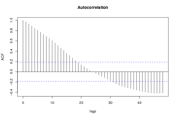
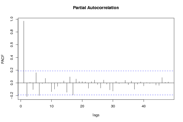
Author's title

Autocorrelation - Koers BEL 20 van Januari 2000 tot Januari 2009 - Claus We...

Author

*Unverified author*

R Software Module

rwasp_autocorrelation.wasp

Title produced by software

(Partial) Autocorrelation Function

Date of computation

Tue, 12 May 2009 07:45:35 -0600

Cite this page as follows

Statistical Computations at FreeStatistics.org, Office for Research Development and Education, URL https://freestatistics.org/blog/index.php?v=date/2009/May/12/t1242136024mua61axzqj0ag1j.htm/, Retrieved Mon, 29 Apr 2024 03:49:02 +0000

Statistical Computations at FreeStatistics.org, Office for Research Development and Education, URL https://freestatistics.org/blog/index.php?pk=39747, Retrieved Mon, 29 Apr 2024 03:49:02 +0000

QR Codes:

Paste this QR Code to cite your computation.

Original text written by user:

IsPrivate?

No (this computation is public)

User-defined keywords

Estimated Impact

177

Family? (F = Feedback message, R = changed R code, M = changed R Module, P = changed Parameters, D = changed Data)

-       [(Partial) Autocorrelation Function] [Autocorrelation -...] [2009-05-12 13:45:35] [fbcf875f1b36dfb87c2c6a55976f6e7b] [Current]

Feedback Forum

Post a new message

Dataseries X:

Download CSV

Histogram

Boxplots

Summary of computational transaction
Raw Input	view raw input (R code)
Raw Output	view raw output of R engine
Computing time	2 seconds
R Server	'Gwilym Jenkins' @ 72.249.127.135

\begin{tabular}{lllllllll}
\hline
Summary of computational transaction \tabularnewline
Raw Input & view raw input (R code)  \tabularnewline
Raw Output & view raw output of R engine  \tabularnewline
Computing time & 2 seconds \tabularnewline
R Server & 'Gwilym Jenkins' @ 72.249.127.135 \tabularnewline
\hline
\end{tabular}
%Source: https://freestatistics.org/blog/index.php?pk=39747&T=0

[TABLE]
[ROW][C]Summary of computational transaction[/C][/ROW]
[ROW][C]Raw Input[/C][C]view raw input (R code) [/C][/ROW]
[ROW][C]Raw Output[/C][C]view raw output of R engine [/C][/ROW]
[ROW][C]Computing time[/C][C]2 seconds[/C][/ROW]
[ROW][C]R Server[/C][C]'Gwilym Jenkins' @ 72.249.127.135[/C][/ROW]
[/TABLE]
Source: https://freestatistics.org/blog/index.php?pk=39747&T=0

Globally Unique Identifier (entire table): ba.freestatistics.org/blog/index.php?pk=39747&T=0

As an alternative you can also use a QR Code:

The GUIDs for individual cells are displayed in the table below:

Summary of computational transaction
Raw Input	view raw input (R code)
Raw Output	view raw output of R engine
Computing time	2 seconds
R Server	'Gwilym Jenkins' @ 72.249.127.135

Autocorrelation Function
Time lag k	ACF(k)	T-STAT	P-value
1	0.971736	10.1452	0
2	0.932321	9.7337	0
3	0.892371	9.3166	0
4	0.848206	8.8555	0
5	0.812086	8.4784	0
6	0.770693	8.0463	0
7	0.725722	7.5768	0
8	0.687153	7.1741	0
9	0.649511	6.7811	0
10	0.608354	6.3514	0
11	0.562464	5.8723	0
12	0.511137	5.3364	0
13	0.460171	4.8043	2e-06
14	0.414713	4.3297	1.7e-05
15	0.365224	3.8131	0.000114
16	0.319092	3.3314	0.00059
17	0.268538	2.8036	0.002992
18	0.217575	2.2716	0.012539
19	0.175983	1.8373	0.034444
20	0.135529	1.415	0.079965
21	0.099338	1.0371	0.150987
22	0.062972	0.6574	0.256139
23	0.025312	0.2643	0.396038
24	-0.004801	-0.0501	0.480056
25	-0.032588	-0.3402	0.367169
26	-0.062234	-0.6497	0.258613
27	-0.090216	-0.9419	0.174168
28	-0.117019	-1.2217	0.112225
29	-0.146452	-1.529	0.064581
30	-0.176177	-1.8393	0.034293
31	-0.207366	-2.165	0.016286
32	-0.238385	-2.4888	0.007165
33	-0.26398	-2.756	0.00343
34	-0.284565	-2.9709	0.001826
35	-0.301183	-3.1444	0.001072
36	-0.314819	-3.2868	0.000682
37	-0.32934	-3.4384	0.000415
38	-0.344447	-3.5961	0.000243
39	-0.358627	-3.7442	0.000145
40	-0.373643	-3.9009	8.3e-05
41	-0.386768	-4.038	5e-05
42	-0.397906	-4.1543	3.3e-05
43	-0.40805	-4.2602	2.2e-05
44	-0.414965	-4.3324	1.6e-05
45	-0.420775	-4.393	1.3e-05
46	-0.422325	-4.4092	1.2e-05
47	-0.420312	-4.3882	1.3e-05
48	-0.415042	-4.3332	1.6e-05

\begin{tabular}{lllllllll}
\hline
Autocorrelation Function \tabularnewline
Time lag k & ACF(k) & T-STAT & P-value \tabularnewline
1 & 0.971736 & 10.1452 & 0 \tabularnewline
2 & 0.932321 & 9.7337 & 0 \tabularnewline
3 & 0.892371 & 9.3166 & 0 \tabularnewline
4 & 0.848206 & 8.8555 & 0 \tabularnewline
5 & 0.812086 & 8.4784 & 0 \tabularnewline
6 & 0.770693 & 8.0463 & 0 \tabularnewline
7 & 0.725722 & 7.5768 & 0 \tabularnewline
8 & 0.687153 & 7.1741 & 0 \tabularnewline
9 & 0.649511 & 6.7811 & 0 \tabularnewline
10 & 0.608354 & 6.3514 & 0 \tabularnewline
11 & 0.562464 & 5.8723 & 0 \tabularnewline
12 & 0.511137 & 5.3364 & 0 \tabularnewline
13 & 0.460171 & 4.8043 & 2e-06 \tabularnewline
14 & 0.414713 & 4.3297 & 1.7e-05 \tabularnewline
15 & 0.365224 & 3.8131 & 0.000114 \tabularnewline
16 & 0.319092 & 3.3314 & 0.00059 \tabularnewline
17 & 0.268538 & 2.8036 & 0.002992 \tabularnewline
18 & 0.217575 & 2.2716 & 0.012539 \tabularnewline
19 & 0.175983 & 1.8373 & 0.034444 \tabularnewline
20 & 0.135529 & 1.415 & 0.079965 \tabularnewline
21 & 0.099338 & 1.0371 & 0.150987 \tabularnewline
22 & 0.062972 & 0.6574 & 0.256139 \tabularnewline
23 & 0.025312 & 0.2643 & 0.396038 \tabularnewline
24 & -0.004801 & -0.0501 & 0.480056 \tabularnewline
25 & -0.032588 & -0.3402 & 0.367169 \tabularnewline
26 & -0.062234 & -0.6497 & 0.258613 \tabularnewline
27 & -0.090216 & -0.9419 & 0.174168 \tabularnewline
28 & -0.117019 & -1.2217 & 0.112225 \tabularnewline
29 & -0.146452 & -1.529 & 0.064581 \tabularnewline
30 & -0.176177 & -1.8393 & 0.034293 \tabularnewline
31 & -0.207366 & -2.165 & 0.016286 \tabularnewline
32 & -0.238385 & -2.4888 & 0.007165 \tabularnewline
33 & -0.26398 & -2.756 & 0.00343 \tabularnewline
34 & -0.284565 & -2.9709 & 0.001826 \tabularnewline
35 & -0.301183 & -3.1444 & 0.001072 \tabularnewline
36 & -0.314819 & -3.2868 & 0.000682 \tabularnewline
37 & -0.32934 & -3.4384 & 0.000415 \tabularnewline
38 & -0.344447 & -3.5961 & 0.000243 \tabularnewline
39 & -0.358627 & -3.7442 & 0.000145 \tabularnewline
40 & -0.373643 & -3.9009 & 8.3e-05 \tabularnewline
41 & -0.386768 & -4.038 & 5e-05 \tabularnewline
42 & -0.397906 & -4.1543 & 3.3e-05 \tabularnewline
43 & -0.40805 & -4.2602 & 2.2e-05 \tabularnewline
44 & -0.414965 & -4.3324 & 1.6e-05 \tabularnewline
45 & -0.420775 & -4.393 & 1.3e-05 \tabularnewline
46 & -0.422325 & -4.4092 & 1.2e-05 \tabularnewline
47 & -0.420312 & -4.3882 & 1.3e-05 \tabularnewline
48 & -0.415042 & -4.3332 & 1.6e-05 \tabularnewline
\hline
\end{tabular}
%Source: https://freestatistics.org/blog/index.php?pk=39747&T=1

[TABLE]
[ROW][C]Autocorrelation Function[/C][/ROW]
[ROW][C]Time lag k[/C][C]ACF(k)[/C][C]T-STAT[/C][C]P-value[/C][/ROW]
[ROW][C]1[/C][C]0.971736[/C][C]10.1452[/C][C]0[/C][/ROW]
[ROW][C]2[/C][C]0.932321[/C][C]9.7337[/C][C]0[/C][/ROW]
[ROW][C]3[/C][C]0.892371[/C][C]9.3166[/C][C]0[/C][/ROW]
[ROW][C]4[/C][C]0.848206[/C][C]8.8555[/C][C]0[/C][/ROW]
[ROW][C]5[/C][C]0.812086[/C][C]8.4784[/C][C]0[/C][/ROW]
[ROW][C]6[/C][C]0.770693[/C][C]8.0463[/C][C]0[/C][/ROW]
[ROW][C]7[/C][C]0.725722[/C][C]7.5768[/C][C]0[/C][/ROW]
[ROW][C]8[/C][C]0.687153[/C][C]7.1741[/C][C]0[/C][/ROW]
[ROW][C]9[/C][C]0.649511[/C][C]6.7811[/C][C]0[/C][/ROW]
[ROW][C]10[/C][C]0.608354[/C][C]6.3514[/C][C]0[/C][/ROW]
[ROW][C]11[/C][C]0.562464[/C][C]5.8723[/C][C]0[/C][/ROW]
[ROW][C]12[/C][C]0.511137[/C][C]5.3364[/C][C]0[/C][/ROW]
[ROW][C]13[/C][C]0.460171[/C][C]4.8043[/C][C]2e-06[/C][/ROW]
[ROW][C]14[/C][C]0.414713[/C][C]4.3297[/C][C]1.7e-05[/C][/ROW]
[ROW][C]15[/C][C]0.365224[/C][C]3.8131[/C][C]0.000114[/C][/ROW]
[ROW][C]16[/C][C]0.319092[/C][C]3.3314[/C][C]0.00059[/C][/ROW]
[ROW][C]17[/C][C]0.268538[/C][C]2.8036[/C][C]0.002992[/C][/ROW]
[ROW][C]18[/C][C]0.217575[/C][C]2.2716[/C][C]0.012539[/C][/ROW]
[ROW][C]19[/C][C]0.175983[/C][C]1.8373[/C][C]0.034444[/C][/ROW]
[ROW][C]20[/C][C]0.135529[/C][C]1.415[/C][C]0.079965[/C][/ROW]
[ROW][C]21[/C][C]0.099338[/C][C]1.0371[/C][C]0.150987[/C][/ROW]
[ROW][C]22[/C][C]0.062972[/C][C]0.6574[/C][C]0.256139[/C][/ROW]
[ROW][C]23[/C][C]0.025312[/C][C]0.2643[/C][C]0.396038[/C][/ROW]
[ROW][C]24[/C][C]-0.004801[/C][C]-0.0501[/C][C]0.480056[/C][/ROW]
[ROW][C]25[/C][C]-0.032588[/C][C]-0.3402[/C][C]0.367169[/C][/ROW]
[ROW][C]26[/C][C]-0.062234[/C][C]-0.6497[/C][C]0.258613[/C][/ROW]
[ROW][C]27[/C][C]-0.090216[/C][C]-0.9419[/C][C]0.174168[/C][/ROW]
[ROW][C]28[/C][C]-0.117019[/C][C]-1.2217[/C][C]0.112225[/C][/ROW]
[ROW][C]29[/C][C]-0.146452[/C][C]-1.529[/C][C]0.064581[/C][/ROW]
[ROW][C]30[/C][C]-0.176177[/C][C]-1.8393[/C][C]0.034293[/C][/ROW]
[ROW][C]31[/C][C]-0.207366[/C][C]-2.165[/C][C]0.016286[/C][/ROW]
[ROW][C]32[/C][C]-0.238385[/C][C]-2.4888[/C][C]0.007165[/C][/ROW]
[ROW][C]33[/C][C]-0.26398[/C][C]-2.756[/C][C]0.00343[/C][/ROW]
[ROW][C]34[/C][C]-0.284565[/C][C]-2.9709[/C][C]0.001826[/C][/ROW]
[ROW][C]35[/C][C]-0.301183[/C][C]-3.1444[/C][C]0.001072[/C][/ROW]
[ROW][C]36[/C][C]-0.314819[/C][C]-3.2868[/C][C]0.000682[/C][/ROW]
[ROW][C]37[/C][C]-0.32934[/C][C]-3.4384[/C][C]0.000415[/C][/ROW]
[ROW][C]38[/C][C]-0.344447[/C][C]-3.5961[/C][C]0.000243[/C][/ROW]
[ROW][C]39[/C][C]-0.358627[/C][C]-3.7442[/C][C]0.000145[/C][/ROW]
[ROW][C]40[/C][C]-0.373643[/C][C]-3.9009[/C][C]8.3e-05[/C][/ROW]
[ROW][C]41[/C][C]-0.386768[/C][C]-4.038[/C][C]5e-05[/C][/ROW]
[ROW][C]42[/C][C]-0.397906[/C][C]-4.1543[/C][C]3.3e-05[/C][/ROW]
[ROW][C]43[/C][C]-0.40805[/C][C]-4.2602[/C][C]2.2e-05[/C][/ROW]
[ROW][C]44[/C][C]-0.414965[/C][C]-4.3324[/C][C]1.6e-05[/C][/ROW]
[ROW][C]45[/C][C]-0.420775[/C][C]-4.393[/C][C]1.3e-05[/C][/ROW]
[ROW][C]46[/C][C]-0.422325[/C][C]-4.4092[/C][C]1.2e-05[/C][/ROW]
[ROW][C]47[/C][C]-0.420312[/C][C]-4.3882[/C][C]1.3e-05[/C][/ROW]
[ROW][C]48[/C][C]-0.415042[/C][C]-4.3332[/C][C]1.6e-05[/C][/ROW]
[/TABLE]
Source: https://freestatistics.org/blog/index.php?pk=39747&T=1

Globally Unique Identifier (entire table): ba.freestatistics.org/blog/index.php?pk=39747&T=1

As an alternative you can also use a QR Code:

The GUIDs for individual cells are displayed in the table below:

Autocorrelation Function
Time lag k	ACF(k)	T-STAT	P-value
1	0.971736	10.1452	0
2	0.932321	9.7337	0
3	0.892371	9.3166	0
4	0.848206	8.8555	0
5	0.812086	8.4784	0
6	0.770693	8.0463	0
7	0.725722	7.5768	0
8	0.687153	7.1741	0
9	0.649511	6.7811	0
10	0.608354	6.3514	0
11	0.562464	5.8723	0
12	0.511137	5.3364	0
13	0.460171	4.8043	2e-06
14	0.414713	4.3297	1.7e-05
15	0.365224	3.8131	0.000114
16	0.319092	3.3314	0.00059
17	0.268538	2.8036	0.002992
18	0.217575	2.2716	0.012539
19	0.175983	1.8373	0.034444
20	0.135529	1.415	0.079965
21	0.099338	1.0371	0.150987
22	0.062972	0.6574	0.256139
23	0.025312	0.2643	0.396038
24	-0.004801	-0.0501	0.480056
25	-0.032588	-0.3402	0.367169
26	-0.062234	-0.6497	0.258613
27	-0.090216	-0.9419	0.174168
28	-0.117019	-1.2217	0.112225
29	-0.146452	-1.529	0.064581
30	-0.176177	-1.8393	0.034293
31	-0.207366	-2.165	0.016286
32	-0.238385	-2.4888	0.007165
33	-0.26398	-2.756	0.00343
34	-0.284565	-2.9709	0.001826
35	-0.301183	-3.1444	0.001072
36	-0.314819	-3.2868	0.000682
37	-0.32934	-3.4384	0.000415
38	-0.344447	-3.5961	0.000243
39	-0.358627	-3.7442	0.000145
40	-0.373643	-3.9009	8.3e-05
41	-0.386768	-4.038	5e-05
42	-0.397906	-4.1543	3.3e-05
43	-0.40805	-4.2602	2.2e-05
44	-0.414965	-4.3324	1.6e-05
45	-0.420775	-4.393	1.3e-05
46	-0.422325	-4.4092	1.2e-05
47	-0.420312	-4.3882	1.3e-05
48	-0.415042	-4.3332	1.6e-05

Partial Autocorrelation Function
Time lag k	PACF(k)	T-STAT	P-value
1	0.971736	10.1452	0
2	-0.214411	-2.2385	0.01361
3	0.009461	0.0988	0.460748
4	-0.104665	-1.0927	0.13846
5	0.161073	1.6816	0.04775
6	-0.198436	-2.0717	0.020325
7	-0.010364	-0.1082	0.457018
8	0.071946	0.7511	0.227093
9	-0.001356	-0.0142	0.494366
10	-0.138539	-1.4464	0.075469
11	-0.097761	-1.0207	0.154838
12	-0.053778	-0.5615	0.287818
13	-0.003631	-0.0379	0.484916
14	0.033376	0.3485	0.364085
15	-0.14744	-1.5393	0.063313
16	0.095033	0.9922	0.161654
17	-0.190709	-1.9911	0.024488
18	0.061758	0.6448	0.260214
19	0.022297	0.2328	0.408183
20	0.021395	0.2234	0.411832
21	0.016197	0.1691	0.433015
22	-0.083827	-0.8752	0.191699
23	0.020121	0.2101	0.417004
24	0.045589	0.476	0.317527
25	-0.02413	-0.2519	0.400788
26	-0.081223	-0.848	0.19915
27	0.046146	0.4818	0.315465
28	-0.019705	-0.2057	0.418694
29	-0.109717	-1.1455	0.127261
30	-0.12817	-1.3381	0.091819
31	0.023477	0.2451	0.403415
32	-0.009841	-0.1027	0.459176
33	-0.000321	-0.0034	0.498666
34	0.041745	0.4358	0.331909
35	-0.027689	-0.2891	0.386535
36	0.029294	0.3058	0.380156
37	-0.099562	-1.0395	0.150446
38	-0.020467	-0.2137	0.415596
39	0.016887	0.1763	0.430191
40	-0.047445	-0.4953	0.31068
41	0.00533	0.0556	0.477861
42	-0.007856	-0.082	0.46739
43	-0.001804	-0.0188	0.492506
44	-0.033684	-0.3517	0.362881
45	-0.039033	-0.4075	0.342212
46	0.084492	0.8821	0.189825
47	0.010616	0.1108	0.455976
48	0.01464	0.1528	0.439403

\begin{tabular}{lllllllll}
\hline
Partial Autocorrelation Function \tabularnewline
Time lag k & PACF(k) & T-STAT & P-value \tabularnewline
1 & 0.971736 & 10.1452 & 0 \tabularnewline
2 & -0.214411 & -2.2385 & 0.01361 \tabularnewline
3 & 0.009461 & 0.0988 & 0.460748 \tabularnewline
4 & -0.104665 & -1.0927 & 0.13846 \tabularnewline
5 & 0.161073 & 1.6816 & 0.04775 \tabularnewline
6 & -0.198436 & -2.0717 & 0.020325 \tabularnewline
7 & -0.010364 & -0.1082 & 0.457018 \tabularnewline
8 & 0.071946 & 0.7511 & 0.227093 \tabularnewline
9 & -0.001356 & -0.0142 & 0.494366 \tabularnewline
10 & -0.138539 & -1.4464 & 0.075469 \tabularnewline
11 & -0.097761 & -1.0207 & 0.154838 \tabularnewline
12 & -0.053778 & -0.5615 & 0.287818 \tabularnewline
13 & -0.003631 & -0.0379 & 0.484916 \tabularnewline
14 & 0.033376 & 0.3485 & 0.364085 \tabularnewline
15 & -0.14744 & -1.5393 & 0.063313 \tabularnewline
16 & 0.095033 & 0.9922 & 0.161654 \tabularnewline
17 & -0.190709 & -1.9911 & 0.024488 \tabularnewline
18 & 0.061758 & 0.6448 & 0.260214 \tabularnewline
19 & 0.022297 & 0.2328 & 0.408183 \tabularnewline
20 & 0.021395 & 0.2234 & 0.411832 \tabularnewline
21 & 0.016197 & 0.1691 & 0.433015 \tabularnewline
22 & -0.083827 & -0.8752 & 0.191699 \tabularnewline
23 & 0.020121 & 0.2101 & 0.417004 \tabularnewline
24 & 0.045589 & 0.476 & 0.317527 \tabularnewline
25 & -0.02413 & -0.2519 & 0.400788 \tabularnewline
26 & -0.081223 & -0.848 & 0.19915 \tabularnewline
27 & 0.046146 & 0.4818 & 0.315465 \tabularnewline
28 & -0.019705 & -0.2057 & 0.418694 \tabularnewline
29 & -0.109717 & -1.1455 & 0.127261 \tabularnewline
30 & -0.12817 & -1.3381 & 0.091819 \tabularnewline
31 & 0.023477 & 0.2451 & 0.403415 \tabularnewline
32 & -0.009841 & -0.1027 & 0.459176 \tabularnewline
33 & -0.000321 & -0.0034 & 0.498666 \tabularnewline
34 & 0.041745 & 0.4358 & 0.331909 \tabularnewline
35 & -0.027689 & -0.2891 & 0.386535 \tabularnewline
36 & 0.029294 & 0.3058 & 0.380156 \tabularnewline
37 & -0.099562 & -1.0395 & 0.150446 \tabularnewline
38 & -0.020467 & -0.2137 & 0.415596 \tabularnewline
39 & 0.016887 & 0.1763 & 0.430191 \tabularnewline
40 & -0.047445 & -0.4953 & 0.31068 \tabularnewline
41 & 0.00533 & 0.0556 & 0.477861 \tabularnewline
42 & -0.007856 & -0.082 & 0.46739 \tabularnewline
43 & -0.001804 & -0.0188 & 0.492506 \tabularnewline
44 & -0.033684 & -0.3517 & 0.362881 \tabularnewline
45 & -0.039033 & -0.4075 & 0.342212 \tabularnewline
46 & 0.084492 & 0.8821 & 0.189825 \tabularnewline
47 & 0.010616 & 0.1108 & 0.455976 \tabularnewline
48 & 0.01464 & 0.1528 & 0.439403 \tabularnewline
\hline
\end{tabular}
%Source: https://freestatistics.org/blog/index.php?pk=39747&T=2

[TABLE]
[ROW][C]Partial Autocorrelation Function[/C][/ROW]
[ROW][C]Time lag k[/C][C]PACF(k)[/C][C]T-STAT[/C][C]P-value[/C][/ROW]
[ROW][C]1[/C][C]0.971736[/C][C]10.1452[/C][C]0[/C][/ROW]
[ROW][C]2[/C][C]-0.214411[/C][C]-2.2385[/C][C]0.01361[/C][/ROW]
[ROW][C]3[/C][C]0.009461[/C][C]0.0988[/C][C]0.460748[/C][/ROW]
[ROW][C]4[/C][C]-0.104665[/C][C]-1.0927[/C][C]0.13846[/C][/ROW]
[ROW][C]5[/C][C]0.161073[/C][C]1.6816[/C][C]0.04775[/C][/ROW]
[ROW][C]6[/C][C]-0.198436[/C][C]-2.0717[/C][C]0.020325[/C][/ROW]
[ROW][C]7[/C][C]-0.010364[/C][C]-0.1082[/C][C]0.457018[/C][/ROW]
[ROW][C]8[/C][C]0.071946[/C][C]0.7511[/C][C]0.227093[/C][/ROW]
[ROW][C]9[/C][C]-0.001356[/C][C]-0.0142[/C][C]0.494366[/C][/ROW]
[ROW][C]10[/C][C]-0.138539[/C][C]-1.4464[/C][C]0.075469[/C][/ROW]
[ROW][C]11[/C][C]-0.097761[/C][C]-1.0207[/C][C]0.154838[/C][/ROW]
[ROW][C]12[/C][C]-0.053778[/C][C]-0.5615[/C][C]0.287818[/C][/ROW]
[ROW][C]13[/C][C]-0.003631[/C][C]-0.0379[/C][C]0.484916[/C][/ROW]
[ROW][C]14[/C][C]0.033376[/C][C]0.3485[/C][C]0.364085[/C][/ROW]
[ROW][C]15[/C][C]-0.14744[/C][C]-1.5393[/C][C]0.063313[/C][/ROW]
[ROW][C]16[/C][C]0.095033[/C][C]0.9922[/C][C]0.161654[/C][/ROW]
[ROW][C]17[/C][C]-0.190709[/C][C]-1.9911[/C][C]0.024488[/C][/ROW]
[ROW][C]18[/C][C]0.061758[/C][C]0.6448[/C][C]0.260214[/C][/ROW]
[ROW][C]19[/C][C]0.022297[/C][C]0.2328[/C][C]0.408183[/C][/ROW]
[ROW][C]20[/C][C]0.021395[/C][C]0.2234[/C][C]0.411832[/C][/ROW]
[ROW][C]21[/C][C]0.016197[/C][C]0.1691[/C][C]0.433015[/C][/ROW]
[ROW][C]22[/C][C]-0.083827[/C][C]-0.8752[/C][C]0.191699[/C][/ROW]
[ROW][C]23[/C][C]0.020121[/C][C]0.2101[/C][C]0.417004[/C][/ROW]
[ROW][C]24[/C][C]0.045589[/C][C]0.476[/C][C]0.317527[/C][/ROW]
[ROW][C]25[/C][C]-0.02413[/C][C]-0.2519[/C][C]0.400788[/C][/ROW]
[ROW][C]26[/C][C]-0.081223[/C][C]-0.848[/C][C]0.19915[/C][/ROW]
[ROW][C]27[/C][C]0.046146[/C][C]0.4818[/C][C]0.315465[/C][/ROW]
[ROW][C]28[/C][C]-0.019705[/C][C]-0.2057[/C][C]0.418694[/C][/ROW]
[ROW][C]29[/C][C]-0.109717[/C][C]-1.1455[/C][C]0.127261[/C][/ROW]
[ROW][C]30[/C][C]-0.12817[/C][C]-1.3381[/C][C]0.091819[/C][/ROW]
[ROW][C]31[/C][C]0.023477[/C][C]0.2451[/C][C]0.403415[/C][/ROW]
[ROW][C]32[/C][C]-0.009841[/C][C]-0.1027[/C][C]0.459176[/C][/ROW]
[ROW][C]33[/C][C]-0.000321[/C][C]-0.0034[/C][C]0.498666[/C][/ROW]
[ROW][C]34[/C][C]0.041745[/C][C]0.4358[/C][C]0.331909[/C][/ROW]
[ROW][C]35[/C][C]-0.027689[/C][C]-0.2891[/C][C]0.386535[/C][/ROW]
[ROW][C]36[/C][C]0.029294[/C][C]0.3058[/C][C]0.380156[/C][/ROW]
[ROW][C]37[/C][C]-0.099562[/C][C]-1.0395[/C][C]0.150446[/C][/ROW]
[ROW][C]38[/C][C]-0.020467[/C][C]-0.2137[/C][C]0.415596[/C][/ROW]
[ROW][C]39[/C][C]0.016887[/C][C]0.1763[/C][C]0.430191[/C][/ROW]
[ROW][C]40[/C][C]-0.047445[/C][C]-0.4953[/C][C]0.31068[/C][/ROW]
[ROW][C]41[/C][C]0.00533[/C][C]0.0556[/C][C]0.477861[/C][/ROW]
[ROW][C]42[/C][C]-0.007856[/C][C]-0.082[/C][C]0.46739[/C][/ROW]
[ROW][C]43[/C][C]-0.001804[/C][C]-0.0188[/C][C]0.492506[/C][/ROW]
[ROW][C]44[/C][C]-0.033684[/C][C]-0.3517[/C][C]0.362881[/C][/ROW]
[ROW][C]45[/C][C]-0.039033[/C][C]-0.4075[/C][C]0.342212[/C][/ROW]
[ROW][C]46[/C][C]0.084492[/C][C]0.8821[/C][C]0.189825[/C][/ROW]
[ROW][C]47[/C][C]0.010616[/C][C]0.1108[/C][C]0.455976[/C][/ROW]
[ROW][C]48[/C][C]0.01464[/C][C]0.1528[/C][C]0.439403[/C][/ROW]
[/TABLE]
Source: https://freestatistics.org/blog/index.php?pk=39747&T=2

Globally Unique Identifier (entire table): ba.freestatistics.org/blog/index.php?pk=39747&T=2

As an alternative you can also use a QR Code:

The GUIDs for individual cells are displayed in the table below:

Partial Autocorrelation Function
Time lag k	PACF(k)	T-STAT	P-value
1	0.971736	10.1452	0
2	-0.214411	-2.2385	0.01361
3	0.009461	0.0988	0.460748
4	-0.104665	-1.0927	0.13846
5	0.161073	1.6816	0.04775
6	-0.198436	-2.0717	0.020325
7	-0.010364	-0.1082	0.457018
8	0.071946	0.7511	0.227093
9	-0.001356	-0.0142	0.494366
10	-0.138539	-1.4464	0.075469
11	-0.097761	-1.0207	0.154838
12	-0.053778	-0.5615	0.287818
13	-0.003631	-0.0379	0.484916
14	0.033376	0.3485	0.364085
15	-0.14744	-1.5393	0.063313
16	0.095033	0.9922	0.161654
17	-0.190709	-1.9911	0.024488
18	0.061758	0.6448	0.260214
19	0.022297	0.2328	0.408183
20	0.021395	0.2234	0.411832
21	0.016197	0.1691	0.433015
22	-0.083827	-0.8752	0.191699
23	0.020121	0.2101	0.417004
24	0.045589	0.476	0.317527
25	-0.02413	-0.2519	0.400788
26	-0.081223	-0.848	0.19915
27	0.046146	0.4818	0.315465
28	-0.019705	-0.2057	0.418694
29	-0.109717	-1.1455	0.127261
30	-0.12817	-1.3381	0.091819
31	0.023477	0.2451	0.403415
32	-0.009841	-0.1027	0.459176
33	-0.000321	-0.0034	0.498666
34	0.041745	0.4358	0.331909
35	-0.027689	-0.2891	0.386535
36	0.029294	0.3058	0.380156
37	-0.099562	-1.0395	0.150446
38	-0.020467	-0.2137	0.415596
39	0.016887	0.1763	0.430191
40	-0.047445	-0.4953	0.31068
41	0.00533	0.0556	0.477861
42	-0.007856	-0.082	0.46739
43	-0.001804	-0.0188	0.492506
44	-0.033684	-0.3517	0.362881
45	-0.039033	-0.4075	0.342212
46	0.084492	0.8821	0.189825
47	0.010616	0.1108	0.455976
48	0.01464	0.1528	0.439403

Figure 1

PNG link

Postscript link

PDF link

Figure 2

PNG link

Postscript link

PDF link

Parameters (Session):

par1 = 48 ; par2 = 1 ; par3 = 0 ; par4 = 0 ; par5 = 12 ;

Parameters (R input):

par1 = 48 ; par2 = 1 ; par3 = 0 ; par4 = 0 ; par5 = 12 ;

R code (references can be found in the software module):

if (par1 == 'Default') {
par1 = 10*log10(length(x))
} else {
par1 <- as.numeric(par1)
}
par2 <- as.numeric(par2)
par3 <- as.numeric(par3)
par4 <- as.numeric(par4)
par5 <- as.numeric(par5)
if (par2 == 0) {
x <- log(x)
} else {
x <- (x ^ par2 - 1) / par2
}
if (par3 > 0) x <- diff(x,lag=1,difference=par3)
if (par4 > 0) x <- diff(x,lag=par5,difference=par4)
bitmap(file='pic1.png')
racf <- acf(x,par1,main='Autocorrelation',xlab='lags',ylab='ACF')
dev.off()
bitmap(file='pic2.png')
rpacf <- pacf(x,par1,main='Partial Autocorrelation',xlab='lags',ylab='PACF')
dev.off()
(myacf <- c(racf$acf))
(mypacf <- c(rpacf$acf))
lengthx <- length(x)
sqrtn <- sqrt(lengthx)
load(file='createtable')
a<-table.start()
a<-table.row.start(a)
a<-table.element(a,'Autocorrelation Function',4,TRUE)
a<-table.row.end(a)
a<-table.row.start(a)
a<-table.element(a,'Time lag k',header=TRUE)
a<-table.element(a,hyperlink('basics.htm','ACF(k)','click here for more information about the Autocorrelation Function'),header=TRUE)
a<-table.element(a,'T-STAT',header=TRUE)
a<-table.element(a,'P-value',header=TRUE)
a<-table.row.end(a)
for (i in 2:(par1+1)) {
a<-table.row.start(a)
a<-table.element(a,i-1,header=TRUE)
a<-table.element(a,round(myacf[i],6))
mytstat <- myacf[i]*sqrtn
a<-table.element(a,round(mytstat,4))
a<-table.element(a,round(1-pt(abs(mytstat),lengthx),6))
a<-table.row.end(a)
}
a<-table.end(a)
table.save(a,file='mytable.tab')
a<-table.start()
a<-table.row.start(a)
a<-table.element(a,'Partial Autocorrelation Function',4,TRUE)
a<-table.row.end(a)
a<-table.row.start(a)
a<-table.element(a,'Time lag k',header=TRUE)
a<-table.element(a,hyperlink('basics.htm','PACF(k)','click here for more information about the Partial Autocorrelation Function'),header=TRUE)
a<-table.element(a,'T-STAT',header=TRUE)
a<-table.element(a,'P-value',header=TRUE)
a<-table.row.end(a)
for (i in 1:par1) {
a<-table.row.start(a)
a<-table.element(a,i,header=TRUE)
a<-table.element(a,round(mypacf[i],6))
mytstat <- mypacf[i]*sqrtn
a<-table.element(a,round(mytstat,4))
a<-table.element(a,round(1-pt(abs(mytstat),lengthx),6))
a<-table.row.end(a)
}
a<-table.end(a)
table.save(a,file='mytable1.tab')

Free Statistics

Description of Statistical Computation

Autocorrelation - Koers BEL 20 van Januari 2000 tot Januari 2009 - Claus We...

Tree of Dependent Computations

Dataset

Tables (Output of Computation)

Figures (Output of Computation)

Input Parameters & R Code