Repository of Reproducible Computations

Free Statistics

of Irreproducible Research!

Author's title

Author

*Unverified author*

R Software Module

rwasp_histogram.wasp

Title produced by software

Histogram

Date of computation

Wed, 04 Mar 2009 04:12:27 -0700

Cite this page as follows

Statistical Computations at FreeStatistics.org, Office for Research Development and Education, URL https://freestatistics.org/blog/index.php?v=date/2009/Mar/04/t1236165386rl3hwfz6wu9u08e.htm/, Retrieved Sat, 27 Apr 2024 23:05:46 +0000

Statistical Computations at FreeStatistics.org, Office for Research Development and Education, URL https://freestatistics.org/blog/index.php?pk=38490, Retrieved Sat, 27 Apr 2024 23:05:46 +0000

QR Codes:

Paste this QR Code to cite your computation.

Original text written by user:

cijfers zijn weergegeven per percent

IsPrivate?

No (this computation is public)

User-defined keywords

historiek en frequentietabel werkloosheidsgraad Belgi� in percentage van de beroepsbevolking

Estimated Impact

187

Family? (F = Feedback message, R = changed R code, M = changed R Module, P = changed Parameters, D = changed Data)

-     [Histogram] [frequentietabel v...] [2009-02-12 13:13:51] [a18c43c8b63fa6800a53bb187b9ddd45]
-   PD    [Histogram] [historiek en freq...] [2009-03-04 11:12:27] [1b767e38463fec58a42ba1ad9c9967aa] [Current]

Feedback Forum

Post a new message

Dataseries X:

Download CSV

Histogram

Boxplots

9.1
9
9
8.9
8.8
8.7
8.5
8.3
8
7.8
7.6
7.6
7.5
7.4
7.2
7
6.8
6.8
6.9
6.9
6.8
6.6
6.5
6.5
6.5
6.5
6.5
6.6
6.6
6.6
6.5
6.6
6.8
7.1
7.1
7.2
7.2
7.2
7.3
7.4
7.5
7.5
7.7
7.7
7.7
7.8
7.9
7.9
8
8.1
8.1
8.3
8.3
8.2
8.1
8.1
8.2
8.3
8.4
8.4
8.4
8.3
8.2
8
8
8.1
8.5
8.6
8.6
8.4
8.4
8.3
8.3
8.4
8.4
8.5
8.5
8.4
8.4
8.4
8.4
8.5
8.5
8.5
8.6
8.6
8.5
8.5
8.4
8.3
8
7.9
8
7.9
8
7.9
7.8
7.7
7.7
7.7
7.7
7.5
7.4
7.3
7.2
7.2
7.1
7.1
7.1
7.1
7
7
6.9
7
7.2
7.2
7.3
7.1
7
7.1

Summary of computational transaction
Raw Input	view raw input (R code)
Raw Output	view raw output of R engine
Computing time	1 seconds
R Server	'Gwilym Jenkins' @ 72.249.127.135

\begin{tabular}{lllllllll}
\hline
Summary of computational transaction \tabularnewline
Raw Input & view raw input (R code)  \tabularnewline
Raw Output & view raw output of R engine  \tabularnewline
Computing time & 1 seconds \tabularnewline
R Server & 'Gwilym Jenkins' @ 72.249.127.135 \tabularnewline
\hline
\end{tabular}
%Source: https://freestatistics.org/blog/index.php?pk=38490&T=0

[TABLE]
[ROW][C]Summary of computational transaction[/C][/ROW]
[ROW][C]Raw Input[/C][C]view raw input (R code) [/C][/ROW]
[ROW][C]Raw Output[/C][C]view raw output of R engine [/C][/ROW]
[ROW][C]Computing time[/C][C]1 seconds[/C][/ROW]
[ROW][C]R Server[/C][C]'Gwilym Jenkins' @ 72.249.127.135[/C][/ROW]
[/TABLE]
Source: https://freestatistics.org/blog/index.php?pk=38490&T=0

Globally Unique Identifier (entire table): ba.freestatistics.org/blog/index.php?pk=38490&T=0

As an alternative you can also use a QR Code:

The GUIDs for individual cells are displayed in the table below:

Summary of computational transaction
Raw Input	view raw input (R code)
Raw Output	view raw output of R engine
Computing time	1 seconds
R Server	'Gwilym Jenkins' @ 72.249.127.135

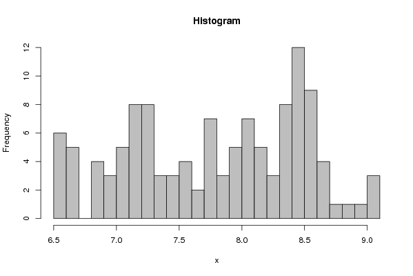
Frequency Table (Histogram)
Bins	Midpoint	Abs. Frequency	Rel. Frequency	Cumul. Rel. Freq.	Density
[6.5,6.6[	6.55	6	0.05	0.05	0.5
[6.6,6.7[	6.65	5	0.041667	0.091667	0.416667
[6.7,6.8[	6.75	0	0	0.091667	0
[6.8,6.9[	6.85	4	0.033333	0.125	0.333333
[6.9,7[	6.95	3	0.025	0.15	0.25
[7,7.1[	7.05	5	0.041667	0.191667	0.416667
[7.1,7.2[	7.15	8	0.066667	0.258333	0.666667
[7.2,7.3[	7.25	8	0.066667	0.325	0.666667
[7.3,7.4[	7.35	3	0.025	0.35	0.25
[7.4,7.5[	7.45	3	0.025	0.375	0.25
[7.5,7.6[	7.55	4	0.033333	0.408333	0.333333
[7.6,7.7[	7.65	2	0.016667	0.425	0.166667
[7.7,7.8[	7.75	7	0.058333	0.483333	0.583333
[7.8,7.9[	7.85	3	0.025	0.508333	0.25
[7.9,8[	7.95	5	0.041667	0.55	0.416667
[8,8.1[	8.05	7	0.058333	0.608333	0.583333
[8.1,8.2[	8.15	5	0.041667	0.65	0.416667
[8.2,8.3[	8.25	3	0.025	0.675	0.25
[8.3,8.4[	8.35	8	0.066667	0.741667	0.666667
[8.4,8.5[	8.45	12	0.1	0.841667	1
[8.5,8.6[	8.55	9	0.075	0.916667	0.75
[8.6,8.7[	8.65	4	0.033333	0.95	0.333333
[8.7,8.8[	8.75	1	0.008333	0.958333	0.083333
[8.8,8.9[	8.85	1	0.008333	0.966667	0.083333
[8.9,9[	8.95	1	0.008333	0.975	0.083333
[9,9.1]	9.05	3	0.025	1	0.25

\begin{tabular}{lllllllll}
\hline
Frequency Table (Histogram) \tabularnewline
Bins & Midpoint & Abs. Frequency & Rel. Frequency & Cumul. Rel. Freq. & Density \tabularnewline
[6.5,6.6[ & 6.55 & 6 & 0.05 & 0.05 & 0.5 \tabularnewline
[6.6,6.7[ & 6.65 & 5 & 0.041667 & 0.091667 & 0.416667 \tabularnewline
[6.7,6.8[ & 6.75 & 0 & 0 & 0.091667 & 0 \tabularnewline
[6.8,6.9[ & 6.85 & 4 & 0.033333 & 0.125 & 0.333333 \tabularnewline
[6.9,7[ & 6.95 & 3 & 0.025 & 0.15 & 0.25 \tabularnewline
[7,7.1[ & 7.05 & 5 & 0.041667 & 0.191667 & 0.416667 \tabularnewline
[7.1,7.2[ & 7.15 & 8 & 0.066667 & 0.258333 & 0.666667 \tabularnewline
[7.2,7.3[ & 7.25 & 8 & 0.066667 & 0.325 & 0.666667 \tabularnewline
[7.3,7.4[ & 7.35 & 3 & 0.025 & 0.35 & 0.25 \tabularnewline
[7.4,7.5[ & 7.45 & 3 & 0.025 & 0.375 & 0.25 \tabularnewline
[7.5,7.6[ & 7.55 & 4 & 0.033333 & 0.408333 & 0.333333 \tabularnewline
[7.6,7.7[ & 7.65 & 2 & 0.016667 & 0.425 & 0.166667 \tabularnewline
[7.7,7.8[ & 7.75 & 7 & 0.058333 & 0.483333 & 0.583333 \tabularnewline
[7.8,7.9[ & 7.85 & 3 & 0.025 & 0.508333 & 0.25 \tabularnewline
[7.9,8[ & 7.95 & 5 & 0.041667 & 0.55 & 0.416667 \tabularnewline
[8,8.1[ & 8.05 & 7 & 0.058333 & 0.608333 & 0.583333 \tabularnewline
[8.1,8.2[ & 8.15 & 5 & 0.041667 & 0.65 & 0.416667 \tabularnewline
[8.2,8.3[ & 8.25 & 3 & 0.025 & 0.675 & 0.25 \tabularnewline
[8.3,8.4[ & 8.35 & 8 & 0.066667 & 0.741667 & 0.666667 \tabularnewline
[8.4,8.5[ & 8.45 & 12 & 0.1 & 0.841667 & 1 \tabularnewline
[8.5,8.6[ & 8.55 & 9 & 0.075 & 0.916667 & 0.75 \tabularnewline
[8.6,8.7[ & 8.65 & 4 & 0.033333 & 0.95 & 0.333333 \tabularnewline
[8.7,8.8[ & 8.75 & 1 & 0.008333 & 0.958333 & 0.083333 \tabularnewline
[8.8,8.9[ & 8.85 & 1 & 0.008333 & 0.966667 & 0.083333 \tabularnewline
[8.9,9[ & 8.95 & 1 & 0.008333 & 0.975 & 0.083333 \tabularnewline
[9,9.1] & 9.05 & 3 & 0.025 & 1 & 0.25 \tabularnewline
\hline
\end{tabular}
%Source: https://freestatistics.org/blog/index.php?pk=38490&T=1

[TABLE]
[ROW][C]Frequency Table (Histogram)[/C][/ROW]
[ROW][C]Bins[/C][C]Midpoint[/C][C]Abs. Frequency[/C][C]Rel. Frequency[/C][C]Cumul. Rel. Freq.[/C][C]Density[/C][/ROW]
[ROW][C][6.5,6.6[[/C][C]6.55[/C][C]6[/C][C]0.05[/C][C]0.05[/C][C]0.5[/C][/ROW]
[ROW][C][6.6,6.7[[/C][C]6.65[/C][C]5[/C][C]0.041667[/C][C]0.091667[/C][C]0.416667[/C][/ROW]
[ROW][C][6.7,6.8[[/C][C]6.75[/C][C]0[/C][C]0[/C][C]0.091667[/C][C]0[/C][/ROW]
[ROW][C][6.8,6.9[[/C][C]6.85[/C][C]4[/C][C]0.033333[/C][C]0.125[/C][C]0.333333[/C][/ROW]
[ROW][C][6.9,7[[/C][C]6.95[/C][C]3[/C][C]0.025[/C][C]0.15[/C][C]0.25[/C][/ROW]
[ROW][C][7,7.1[[/C][C]7.05[/C][C]5[/C][C]0.041667[/C][C]0.191667[/C][C]0.416667[/C][/ROW]
[ROW][C][7.1,7.2[[/C][C]7.15[/C][C]8[/C][C]0.066667[/C][C]0.258333[/C][C]0.666667[/C][/ROW]
[ROW][C][7.2,7.3[[/C][C]7.25[/C][C]8[/C][C]0.066667[/C][C]0.325[/C][C]0.666667[/C][/ROW]
[ROW][C][7.3,7.4[[/C][C]7.35[/C][C]3[/C][C]0.025[/C][C]0.35[/C][C]0.25[/C][/ROW]
[ROW][C][7.4,7.5[[/C][C]7.45[/C][C]3[/C][C]0.025[/C][C]0.375[/C][C]0.25[/C][/ROW]
[ROW][C][7.5,7.6[[/C][C]7.55[/C][C]4[/C][C]0.033333[/C][C]0.408333[/C][C]0.333333[/C][/ROW]
[ROW][C][7.6,7.7[[/C][C]7.65[/C][C]2[/C][C]0.016667[/C][C]0.425[/C][C]0.166667[/C][/ROW]
[ROW][C][7.7,7.8[[/C][C]7.75[/C][C]7[/C][C]0.058333[/C][C]0.483333[/C][C]0.583333[/C][/ROW]
[ROW][C][7.8,7.9[[/C][C]7.85[/C][C]3[/C][C]0.025[/C][C]0.508333[/C][C]0.25[/C][/ROW]
[ROW][C][7.9,8[[/C][C]7.95[/C][C]5[/C][C]0.041667[/C][C]0.55[/C][C]0.416667[/C][/ROW]
[ROW][C][8,8.1[[/C][C]8.05[/C][C]7[/C][C]0.058333[/C][C]0.608333[/C][C]0.583333[/C][/ROW]
[ROW][C][8.1,8.2[[/C][C]8.15[/C][C]5[/C][C]0.041667[/C][C]0.65[/C][C]0.416667[/C][/ROW]
[ROW][C][8.2,8.3[[/C][C]8.25[/C][C]3[/C][C]0.025[/C][C]0.675[/C][C]0.25[/C][/ROW]
[ROW][C][8.3,8.4[[/C][C]8.35[/C][C]8[/C][C]0.066667[/C][C]0.741667[/C][C]0.666667[/C][/ROW]
[ROW][C][8.4,8.5[[/C][C]8.45[/C][C]12[/C][C]0.1[/C][C]0.841667[/C][C]1[/C][/ROW]
[ROW][C][8.5,8.6[[/C][C]8.55[/C][C]9[/C][C]0.075[/C][C]0.916667[/C][C]0.75[/C][/ROW]
[ROW][C][8.6,8.7[[/C][C]8.65[/C][C]4[/C][C]0.033333[/C][C]0.95[/C][C]0.333333[/C][/ROW]
[ROW][C][8.7,8.8[[/C][C]8.75[/C][C]1[/C][C]0.008333[/C][C]0.958333[/C][C]0.083333[/C][/ROW]
[ROW][C][8.8,8.9[[/C][C]8.85[/C][C]1[/C][C]0.008333[/C][C]0.966667[/C][C]0.083333[/C][/ROW]
[ROW][C][8.9,9[[/C][C]8.95[/C][C]1[/C][C]0.008333[/C][C]0.975[/C][C]0.083333[/C][/ROW]
[ROW][C][9,9.1][/C][C]9.05[/C][C]3[/C][C]0.025[/C][C]1[/C][C]0.25[/C][/ROW]
[/TABLE]
Source: https://freestatistics.org/blog/index.php?pk=38490&T=1

Globally Unique Identifier (entire table): ba.freestatistics.org/blog/index.php?pk=38490&T=1

As an alternative you can also use a QR Code:

The GUIDs for individual cells are displayed in the table below:

Frequency Table (Histogram)
Bins	Midpoint	Abs. Frequency	Rel. Frequency	Cumul. Rel. Freq.	Density
[6.5,6.6[	6.55	6	0.05	0.05	0.5
[6.6,6.7[	6.65	5	0.041667	0.091667	0.416667
[6.7,6.8[	6.75	0	0	0.091667	0
[6.8,6.9[	6.85	4	0.033333	0.125	0.333333
[6.9,7[	6.95	3	0.025	0.15	0.25
[7,7.1[	7.05	5	0.041667	0.191667	0.416667
[7.1,7.2[	7.15	8	0.066667	0.258333	0.666667
[7.2,7.3[	7.25	8	0.066667	0.325	0.666667
[7.3,7.4[	7.35	3	0.025	0.35	0.25
[7.4,7.5[	7.45	3	0.025	0.375	0.25
[7.5,7.6[	7.55	4	0.033333	0.408333	0.333333
[7.6,7.7[	7.65	2	0.016667	0.425	0.166667
[7.7,7.8[	7.75	7	0.058333	0.483333	0.583333
[7.8,7.9[	7.85	3	0.025	0.508333	0.25
[7.9,8[	7.95	5	0.041667	0.55	0.416667
[8,8.1[	8.05	7	0.058333	0.608333	0.583333
[8.1,8.2[	8.15	5	0.041667	0.65	0.416667
[8.2,8.3[	8.25	3	0.025	0.675	0.25
[8.3,8.4[	8.35	8	0.066667	0.741667	0.666667
[8.4,8.5[	8.45	12	0.1	0.841667	1
[8.5,8.6[	8.55	9	0.075	0.916667	0.75
[8.6,8.7[	8.65	4	0.033333	0.95	0.333333
[8.7,8.8[	8.75	1	0.008333	0.958333	0.083333
[8.8,8.9[	8.85	1	0.008333	0.966667	0.083333
[8.9,9[	8.95	1	0.008333	0.975	0.083333
[9,9.1]	9.05	3	0.025	1	0.25

Figure 1

PNG link

Postscript link

PDF link

Parameters (Session):

par1 = 30 ; par2 = grey ; par3 = FALSE ; par4 = Unknown ;

Parameters (R input):

par1 = 30 ; par2 = grey ; par3 = FALSE ; par4 = Unknown ;

R code (references can be found in the software module):

par1 <- as.numeric(par1)
if (par3 == 'TRUE') par3 <- TRUE
if (par3 == 'FALSE') par3 <- FALSE
if (par4 == 'Unknown') par1 <- as.numeric(par1)
if (par4 == 'Interval/Ratio') par1 <- as.numeric(par1)
if (par4 == '3-point Likert') par1 <- c(1:3 - 0.5, 3.5)
if (par4 == '4-point Likert') par1 <- c(1:4 - 0.5, 4.5)
if (par4 == '5-point Likert') par1 <- c(1:5 - 0.5, 5.5)
if (par4 == '6-point Likert') par1 <- c(1:6 - 0.5, 6.5)
if (par4 == '7-point Likert') par1 <- c(1:7 - 0.5, 7.5)
if (par4 == '8-point Likert') par1 <- c(1:8 - 0.5, 8.5)
if (par4 == '9-point Likert') par1 <- c(1:9 - 0.5, 9.5)
if (par4 == '10-point Likert') par1 <- c(1:10 - 0.5, 10.5)
bitmap(file='test1.png')
if (is.na(par1)) {
myhist<-hist(x,col=par2,main=main,xlab=xlab,right=par3)
} else {
if (par1 < 0) par1 <- 3
if (par1 > 50) par1 <- 50
myhist<-hist(x,breaks=par1,col=par2,main=main,xlab=xlab,right=par3)
}
dev.off()
myhist
n <- length(x)
load(file='createtable')
a<-table.start()
a<-table.row.start(a)
a<-table.element(a,hyperlink('histogram.htm','Frequency Table (Histogram)',''),6,TRUE)
a<-table.row.end(a)
a<-table.row.start(a)
a<-table.element(a,'Bins',header=TRUE)
a<-table.element(a,'Midpoint',header=TRUE)
a<-table.element(a,'Abs. Frequency',header=TRUE)
a<-table.element(a,'Rel. Frequency',header=TRUE)
a<-table.element(a,'Cumul. Rel. Freq.',header=TRUE)
a<-table.element(a,'Density',header=TRUE)
a<-table.row.end(a)
crf <- 0
if (par3 == FALSE) mybracket <- '[' else mybracket <- ']'
mynumrows <- (length(myhist$breaks)-1)
for (i in 1:mynumrows) {
a<-table.row.start(a)
if (i == 1)
dum <- paste('[',myhist$breaks[i],sep='')
else
dum <- paste(mybracket,myhist$breaks[i],sep='')
dum <- paste(dum,myhist$breaks[i+1],sep=',')
if (i==mynumrows)
dum <- paste(dum,']',sep='')
else
dum <- paste(dum,mybracket,sep='')
a<-table.element(a,dum,header=TRUE)
a<-table.element(a,myhist$mids[i])
a<-table.element(a,myhist$counts[i])
rf <- myhist$counts[i]/n
crf <- crf + rf
a<-table.element(a,round(rf,6))
a<-table.element(a,round(crf,6))
a<-table.element(a,round(myhist$density[i],6))
a<-table.row.end(a)
}
a<-table.end(a)
table.save(a,file='mytable.tab')

Free Statistics

Description of Statistical Computation

Tree of Dependent Computations

Dataset

Tables (Output of Computation)

Figures (Output of Computation)

Input Parameters & R Code