Repository of Reproducible Computations

Free Statistics

of Irreproducible Research!

Author's title

Author

*Unverified author*

R Software Module

rwasp_autocorrelation.wasp

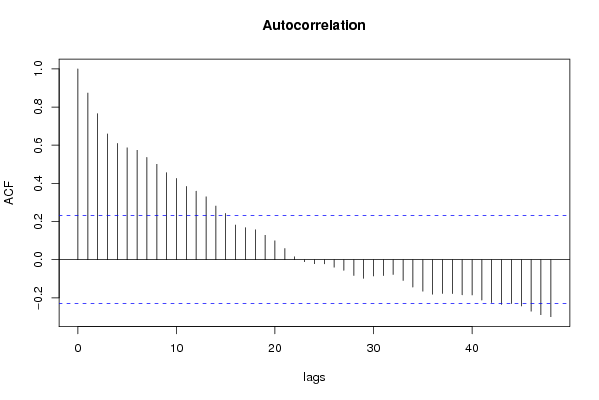
Title produced by software

(Partial) Autocorrelation Function

Date of computation

Sat, 06 Jun 2009 12:14:07 -0600

Cite this page as follows

Statistical Computations at FreeStatistics.org, Office for Research Development and Education, URL https://freestatistics.org/blog/index.php?v=date/2009/Jun/06/t12443120934gxkbblxlu1567o.htm/, Retrieved Mon, 29 Apr 2024 04:04:09 +0000

Statistical Computations at FreeStatistics.org, Office for Research Development and Education, URL https://freestatistics.org/blog/index.php?pk=42045, Retrieved Mon, 29 Apr 2024 04:04:09 +0000

QR Codes:

Paste this QR Code to cite your computation.

Original text written by user:

IsPrivate?

No (this computation is public)

User-defined keywords

Estimated Impact

172

Family? (F = Feedback message, R = changed R code, M = changed R Module, P = changed Parameters, D = changed Data)

-     [(Partial) Autocorrelation Function] [inschrijving nieu...] [2009-06-04 10:51:18] [ef653b42671acc8de32235b938c43afe]
-    D    [(Partial) Autocorrelation Function] [Bruto schuld van ...] [2009-06-06 18:14:07] [2eea656d1ea82c4ced0e8e79cdac0617] [Current]
-           [(Partial) Autocorrelation Function] [Bruto schuld van ...] [2009-06-06 18:16:16] [ef653b42671acc8de32235b938c43afe] 
- RM        [Blocked Bootstrap Plot - Central Tendency] [Bruto schuld van ...] [2009-06-06 18:33:07] [ef653b42671acc8de32235b938c43afe] 
-             [Blocked Bootstrap Plot - Central Tendency] [Bruto schuld van ...] [2009-06-06 18:36:09] [ef653b42671acc8de32235b938c43afe] 
-               [Blocked Bootstrap Plot - Central Tendency] [Bruto schuld van ...] [2009-06-06 18:37:23] [ef653b42671acc8de32235b938c43afe] 
-                 [Blocked Bootstrap Plot - Central Tendency] [Bruto schuld van ...] [2009-06-06 18:39:07] [ef653b42671acc8de32235b938c43afe] 

Feedback Forum

Post a new message

Dataseries X:

Download CSV

Histogram

Boxplots

Summary of computational transaction
Raw Input	view raw input (R code)
Raw Output	view raw output of R engine
Computing time	1 seconds
R Server	'George Udny Yule' @ 72.249.76.132

\begin{tabular}{lllllllll}
\hline
Summary of computational transaction \tabularnewline
Raw Input & view raw input (R code)  \tabularnewline
Raw Output & view raw output of R engine  \tabularnewline
Computing time & 1 seconds \tabularnewline
R Server & 'George Udny Yule' @ 72.249.76.132 \tabularnewline
\hline
\end{tabular}
%Source: https://freestatistics.org/blog/index.php?pk=42045&T=0

[TABLE]
[ROW][C]Summary of computational transaction[/C][/ROW]
[ROW][C]Raw Input[/C][C]view raw input (R code) [/C][/ROW]
[ROW][C]Raw Output[/C][C]view raw output of R engine [/C][/ROW]
[ROW][C]Computing time[/C][C]1 seconds[/C][/ROW]
[ROW][C]R Server[/C][C]'George Udny Yule' @ 72.249.76.132[/C][/ROW]
[/TABLE]
Source: https://freestatistics.org/blog/index.php?pk=42045&T=0

Globally Unique Identifier (entire table): ba.freestatistics.org/blog/index.php?pk=42045&T=0

As an alternative you can also use a QR Code:

The GUIDs for individual cells are displayed in the table below:

Summary of computational transaction
Raw Input	view raw input (R code)
Raw Output	view raw output of R engine
Computing time	1 seconds
R Server	'George Udny Yule' @ 72.249.76.132

Autocorrelation Function
Time lag k	ACF(k)	T-STAT	P-value
1	0.873356	7.4107	0
2	0.765377	6.4944	0
3	0.659446	5.5956	0
4	0.609442	5.1713	1e-06
5	0.586672	4.9781	2e-06
6	0.573145	4.8633	3e-06
7	0.536187	4.5497	1.1e-05
8	0.500007	4.2427	3.2e-05
9	0.455883	3.8683	0.000119
10	0.425872	3.6136	0.000278
11	0.383781	3.2565	0.000861
12	0.359345	3.0491	0.001605
13	0.329648	2.7972	0.003304
14	0.280936	2.3838	0.009886
15	0.242644	2.0589	0.021561
16	0.181345	1.5388	0.064122
17	0.167766	1.4235	0.079449
18	0.15671	1.3297	0.093903
19	0.127574	1.0825	0.141321
20	0.098858	0.8388	0.202168
21	0.058496	0.4964	0.310578
22	0.015062	0.1278	0.449329
23	-0.01029	-0.0873	0.465333
24	-0.020998	-0.1782	0.429545
25	-0.02199	-0.1866	0.426253
26	-0.039444	-0.3347	0.369415
27	-0.055802	-0.4735	0.318647
28	-0.082522	-0.7002	0.243023
29	-0.097521	-0.8275	0.205347
30	-0.085352	-0.7242	0.235635
31	-0.083313	-0.7069	0.240944
32	-0.077797	-0.6601	0.255639
33	-0.109106	-0.9258	0.178824
34	-0.143573	-1.2183	0.113552
35	-0.165242	-1.4021	0.082587
36	-0.180695	-1.5333	0.064798
37	-0.176769	-1.4999	0.069002
38	-0.177547	-1.5065	0.068152
39	-0.184001	-1.5613	0.061419
40	-0.185086	-1.5705	0.060341
41	-0.211974	-1.7987	0.038132
42	-0.225246	-1.9113	0.029975
43	-0.234899	-1.9932	0.025016
44	-0.230251	-1.9537	0.027308
45	-0.242627	-2.0588	0.021568
46	-0.27044	-2.2948	0.012332
47	-0.288849	-2.451	0.008338
48	-0.298805	-2.5354	0.006701

\begin{tabular}{lllllllll}
\hline
Autocorrelation Function \tabularnewline
Time lag k & ACF(k) & T-STAT & P-value \tabularnewline
1 & 0.873356 & 7.4107 & 0 \tabularnewline
2 & 0.765377 & 6.4944 & 0 \tabularnewline
3 & 0.659446 & 5.5956 & 0 \tabularnewline
4 & 0.609442 & 5.1713 & 1e-06 \tabularnewline
5 & 0.586672 & 4.9781 & 2e-06 \tabularnewline
6 & 0.573145 & 4.8633 & 3e-06 \tabularnewline
7 & 0.536187 & 4.5497 & 1.1e-05 \tabularnewline
8 & 0.500007 & 4.2427 & 3.2e-05 \tabularnewline
9 & 0.455883 & 3.8683 & 0.000119 \tabularnewline
10 & 0.425872 & 3.6136 & 0.000278 \tabularnewline
11 & 0.383781 & 3.2565 & 0.000861 \tabularnewline
12 & 0.359345 & 3.0491 & 0.001605 \tabularnewline
13 & 0.329648 & 2.7972 & 0.003304 \tabularnewline
14 & 0.280936 & 2.3838 & 0.009886 \tabularnewline
15 & 0.242644 & 2.0589 & 0.021561 \tabularnewline
16 & 0.181345 & 1.5388 & 0.064122 \tabularnewline
17 & 0.167766 & 1.4235 & 0.079449 \tabularnewline
18 & 0.15671 & 1.3297 & 0.093903 \tabularnewline
19 & 0.127574 & 1.0825 & 0.141321 \tabularnewline
20 & 0.098858 & 0.8388 & 0.202168 \tabularnewline
21 & 0.058496 & 0.4964 & 0.310578 \tabularnewline
22 & 0.015062 & 0.1278 & 0.449329 \tabularnewline
23 & -0.01029 & -0.0873 & 0.465333 \tabularnewline
24 & -0.020998 & -0.1782 & 0.429545 \tabularnewline
25 & -0.02199 & -0.1866 & 0.426253 \tabularnewline
26 & -0.039444 & -0.3347 & 0.369415 \tabularnewline
27 & -0.055802 & -0.4735 & 0.318647 \tabularnewline
28 & -0.082522 & -0.7002 & 0.243023 \tabularnewline
29 & -0.097521 & -0.8275 & 0.205347 \tabularnewline
30 & -0.085352 & -0.7242 & 0.235635 \tabularnewline
31 & -0.083313 & -0.7069 & 0.240944 \tabularnewline
32 & -0.077797 & -0.6601 & 0.255639 \tabularnewline
33 & -0.109106 & -0.9258 & 0.178824 \tabularnewline
34 & -0.143573 & -1.2183 & 0.113552 \tabularnewline
35 & -0.165242 & -1.4021 & 0.082587 \tabularnewline
36 & -0.180695 & -1.5333 & 0.064798 \tabularnewline
37 & -0.176769 & -1.4999 & 0.069002 \tabularnewline
38 & -0.177547 & -1.5065 & 0.068152 \tabularnewline
39 & -0.184001 & -1.5613 & 0.061419 \tabularnewline
40 & -0.185086 & -1.5705 & 0.060341 \tabularnewline
41 & -0.211974 & -1.7987 & 0.038132 \tabularnewline
42 & -0.225246 & -1.9113 & 0.029975 \tabularnewline
43 & -0.234899 & -1.9932 & 0.025016 \tabularnewline
44 & -0.230251 & -1.9537 & 0.027308 \tabularnewline
45 & -0.242627 & -2.0588 & 0.021568 \tabularnewline
46 & -0.27044 & -2.2948 & 0.012332 \tabularnewline
47 & -0.288849 & -2.451 & 0.008338 \tabularnewline
48 & -0.298805 & -2.5354 & 0.006701 \tabularnewline
\hline
\end{tabular}
%Source: https://freestatistics.org/blog/index.php?pk=42045&T=1

[TABLE]
[ROW][C]Autocorrelation Function[/C][/ROW]
[ROW][C]Time lag k[/C][C]ACF(k)[/C][C]T-STAT[/C][C]P-value[/C][/ROW]
[ROW][C]1[/C][C]0.873356[/C][C]7.4107[/C][C]0[/C][/ROW]
[ROW][C]2[/C][C]0.765377[/C][C]6.4944[/C][C]0[/C][/ROW]
[ROW][C]3[/C][C]0.659446[/C][C]5.5956[/C][C]0[/C][/ROW]
[ROW][C]4[/C][C]0.609442[/C][C]5.1713[/C][C]1e-06[/C][/ROW]
[ROW][C]5[/C][C]0.586672[/C][C]4.9781[/C][C]2e-06[/C][/ROW]
[ROW][C]6[/C][C]0.573145[/C][C]4.8633[/C][C]3e-06[/C][/ROW]
[ROW][C]7[/C][C]0.536187[/C][C]4.5497[/C][C]1.1e-05[/C][/ROW]
[ROW][C]8[/C][C]0.500007[/C][C]4.2427[/C][C]3.2e-05[/C][/ROW]
[ROW][C]9[/C][C]0.455883[/C][C]3.8683[/C][C]0.000119[/C][/ROW]
[ROW][C]10[/C][C]0.425872[/C][C]3.6136[/C][C]0.000278[/C][/ROW]
[ROW][C]11[/C][C]0.383781[/C][C]3.2565[/C][C]0.000861[/C][/ROW]
[ROW][C]12[/C][C]0.359345[/C][C]3.0491[/C][C]0.001605[/C][/ROW]
[ROW][C]13[/C][C]0.329648[/C][C]2.7972[/C][C]0.003304[/C][/ROW]
[ROW][C]14[/C][C]0.280936[/C][C]2.3838[/C][C]0.009886[/C][/ROW]
[ROW][C]15[/C][C]0.242644[/C][C]2.0589[/C][C]0.021561[/C][/ROW]
[ROW][C]16[/C][C]0.181345[/C][C]1.5388[/C][C]0.064122[/C][/ROW]
[ROW][C]17[/C][C]0.167766[/C][C]1.4235[/C][C]0.079449[/C][/ROW]
[ROW][C]18[/C][C]0.15671[/C][C]1.3297[/C][C]0.093903[/C][/ROW]
[ROW][C]19[/C][C]0.127574[/C][C]1.0825[/C][C]0.141321[/C][/ROW]
[ROW][C]20[/C][C]0.098858[/C][C]0.8388[/C][C]0.202168[/C][/ROW]
[ROW][C]21[/C][C]0.058496[/C][C]0.4964[/C][C]0.310578[/C][/ROW]
[ROW][C]22[/C][C]0.015062[/C][C]0.1278[/C][C]0.449329[/C][/ROW]
[ROW][C]23[/C][C]-0.01029[/C][C]-0.0873[/C][C]0.465333[/C][/ROW]
[ROW][C]24[/C][C]-0.020998[/C][C]-0.1782[/C][C]0.429545[/C][/ROW]
[ROW][C]25[/C][C]-0.02199[/C][C]-0.1866[/C][C]0.426253[/C][/ROW]
[ROW][C]26[/C][C]-0.039444[/C][C]-0.3347[/C][C]0.369415[/C][/ROW]
[ROW][C]27[/C][C]-0.055802[/C][C]-0.4735[/C][C]0.318647[/C][/ROW]
[ROW][C]28[/C][C]-0.082522[/C][C]-0.7002[/C][C]0.243023[/C][/ROW]
[ROW][C]29[/C][C]-0.097521[/C][C]-0.8275[/C][C]0.205347[/C][/ROW]
[ROW][C]30[/C][C]-0.085352[/C][C]-0.7242[/C][C]0.235635[/C][/ROW]
[ROW][C]31[/C][C]-0.083313[/C][C]-0.7069[/C][C]0.240944[/C][/ROW]
[ROW][C]32[/C][C]-0.077797[/C][C]-0.6601[/C][C]0.255639[/C][/ROW]
[ROW][C]33[/C][C]-0.109106[/C][C]-0.9258[/C][C]0.178824[/C][/ROW]
[ROW][C]34[/C][C]-0.143573[/C][C]-1.2183[/C][C]0.113552[/C][/ROW]
[ROW][C]35[/C][C]-0.165242[/C][C]-1.4021[/C][C]0.082587[/C][/ROW]
[ROW][C]36[/C][C]-0.180695[/C][C]-1.5333[/C][C]0.064798[/C][/ROW]
[ROW][C]37[/C][C]-0.176769[/C][C]-1.4999[/C][C]0.069002[/C][/ROW]
[ROW][C]38[/C][C]-0.177547[/C][C]-1.5065[/C][C]0.068152[/C][/ROW]
[ROW][C]39[/C][C]-0.184001[/C][C]-1.5613[/C][C]0.061419[/C][/ROW]
[ROW][C]40[/C][C]-0.185086[/C][C]-1.5705[/C][C]0.060341[/C][/ROW]
[ROW][C]41[/C][C]-0.211974[/C][C]-1.7987[/C][C]0.038132[/C][/ROW]
[ROW][C]42[/C][C]-0.225246[/C][C]-1.9113[/C][C]0.029975[/C][/ROW]
[ROW][C]43[/C][C]-0.234899[/C][C]-1.9932[/C][C]0.025016[/C][/ROW]
[ROW][C]44[/C][C]-0.230251[/C][C]-1.9537[/C][C]0.027308[/C][/ROW]
[ROW][C]45[/C][C]-0.242627[/C][C]-2.0588[/C][C]0.021568[/C][/ROW]
[ROW][C]46[/C][C]-0.27044[/C][C]-2.2948[/C][C]0.012332[/C][/ROW]
[ROW][C]47[/C][C]-0.288849[/C][C]-2.451[/C][C]0.008338[/C][/ROW]
[ROW][C]48[/C][C]-0.298805[/C][C]-2.5354[/C][C]0.006701[/C][/ROW]
[/TABLE]
Source: https://freestatistics.org/blog/index.php?pk=42045&T=1

Globally Unique Identifier (entire table): ba.freestatistics.org/blog/index.php?pk=42045&T=1

As an alternative you can also use a QR Code:

The GUIDs for individual cells are displayed in the table below:

Autocorrelation Function
Time lag k	ACF(k)	T-STAT	P-value
1	0.873356	7.4107	0
2	0.765377	6.4944	0
3	0.659446	5.5956	0
4	0.609442	5.1713	1e-06
5	0.586672	4.9781	2e-06
6	0.573145	4.8633	3e-06
7	0.536187	4.5497	1.1e-05
8	0.500007	4.2427	3.2e-05
9	0.455883	3.8683	0.000119
10	0.425872	3.6136	0.000278
11	0.383781	3.2565	0.000861
12	0.359345	3.0491	0.001605
13	0.329648	2.7972	0.003304
14	0.280936	2.3838	0.009886
15	0.242644	2.0589	0.021561
16	0.181345	1.5388	0.064122
17	0.167766	1.4235	0.079449
18	0.15671	1.3297	0.093903
19	0.127574	1.0825	0.141321
20	0.098858	0.8388	0.202168
21	0.058496	0.4964	0.310578
22	0.015062	0.1278	0.449329
23	-0.01029	-0.0873	0.465333
24	-0.020998	-0.1782	0.429545
25	-0.02199	-0.1866	0.426253
26	-0.039444	-0.3347	0.369415
27	-0.055802	-0.4735	0.318647
28	-0.082522	-0.7002	0.243023
29	-0.097521	-0.8275	0.205347
30	-0.085352	-0.7242	0.235635
31	-0.083313	-0.7069	0.240944
32	-0.077797	-0.6601	0.255639
33	-0.109106	-0.9258	0.178824
34	-0.143573	-1.2183	0.113552
35	-0.165242	-1.4021	0.082587
36	-0.180695	-1.5333	0.064798
37	-0.176769	-1.4999	0.069002
38	-0.177547	-1.5065	0.068152
39	-0.184001	-1.5613	0.061419
40	-0.185086	-1.5705	0.060341
41	-0.211974	-1.7987	0.038132
42	-0.225246	-1.9113	0.029975
43	-0.234899	-1.9932	0.025016
44	-0.230251	-1.9537	0.027308
45	-0.242627	-2.0588	0.021568
46	-0.27044	-2.2948	0.012332
47	-0.288849	-2.451	0.008338
48	-0.298805	-2.5354	0.006701

Partial Autocorrelation Function
Time lag k	PACF(k)	T-STAT	P-value
1	0.873356	7.4107	0
2	0.011067	0.0939	0.462722
3	-0.047504	-0.4031	0.344039
4	0.173873	1.4754	0.072238
5	0.11363	0.9642	0.169091
6	0.044832	0.3804	0.35238
7	-0.054535	-0.4627	0.322472
8	0.027275	0.2314	0.408815
9	-0.015452	-0.1311	0.448025
10	0.018471	0.1567	0.437947
11	-0.070603	-0.5991	0.275497
12	0.035658	0.3026	0.381545
13	-0.012343	-0.1047	0.458438
14	-0.121161	-1.0281	0.153676
15	0.017253	0.1464	0.442009
16	-0.126479	-1.0732	0.14338
17	0.133473	1.1326	0.130579
18	-0.002886	-0.0245	0.490265
19	-0.124816	-1.0591	0.146547
20	0.02637	0.2238	0.411791
21	-0.039945	-0.3389	0.36782
22	-0.056452	-0.479	0.31669
23	0.002213	0.0188	0.492535
24	0.049513	0.4201	0.33782
25	0.006855	0.0582	0.476887
26	-0.048005	-0.4073	0.342484
27	-0.005916	-0.0502	0.48005
28	-0.022562	-0.1914	0.424359
29	0.043928	0.3727	0.355217
30	0.050572	0.4291	0.33456
31	-0.027286	-0.2315	0.408779
32	0.010034	0.0851	0.466192
33	-0.12407	-1.0528	0.147984
34	-0.01252	-0.1062	0.457846
35	-0.011267	-0.0956	0.462052
36	-0.045295	-0.3843	0.35093
37	0.036466	0.3094	0.378945
38	-0.059918	-0.5084	0.306357
39	-0.006304	-0.0535	0.478745
40	0.036653	0.311	0.378346
41	-0.10632	-0.9022	0.184991
42	-0.015758	-0.1337	0.447001
43	0.014814	0.1257	0.450159
44	0.005968	0.0506	0.479878
45	-0.121253	-1.0289	0.153493
46	-0.037682	-0.3197	0.375046
47	0.015979	0.1356	0.446262
48	0.003173	0.0269	0.489299

\begin{tabular}{lllllllll}
\hline
Partial Autocorrelation Function \tabularnewline
Time lag k & PACF(k) & T-STAT & P-value \tabularnewline
1 & 0.873356 & 7.4107 & 0 \tabularnewline
2 & 0.011067 & 0.0939 & 0.462722 \tabularnewline
3 & -0.047504 & -0.4031 & 0.344039 \tabularnewline
4 & 0.173873 & 1.4754 & 0.072238 \tabularnewline
5 & 0.11363 & 0.9642 & 0.169091 \tabularnewline
6 & 0.044832 & 0.3804 & 0.35238 \tabularnewline
7 & -0.054535 & -0.4627 & 0.322472 \tabularnewline
8 & 0.027275 & 0.2314 & 0.408815 \tabularnewline
9 & -0.015452 & -0.1311 & 0.448025 \tabularnewline
10 & 0.018471 & 0.1567 & 0.437947 \tabularnewline
11 & -0.070603 & -0.5991 & 0.275497 \tabularnewline
12 & 0.035658 & 0.3026 & 0.381545 \tabularnewline
13 & -0.012343 & -0.1047 & 0.458438 \tabularnewline
14 & -0.121161 & -1.0281 & 0.153676 \tabularnewline
15 & 0.017253 & 0.1464 & 0.442009 \tabularnewline
16 & -0.126479 & -1.0732 & 0.14338 \tabularnewline
17 & 0.133473 & 1.1326 & 0.130579 \tabularnewline
18 & -0.002886 & -0.0245 & 0.490265 \tabularnewline
19 & -0.124816 & -1.0591 & 0.146547 \tabularnewline
20 & 0.02637 & 0.2238 & 0.411791 \tabularnewline
21 & -0.039945 & -0.3389 & 0.36782 \tabularnewline
22 & -0.056452 & -0.479 & 0.31669 \tabularnewline
23 & 0.002213 & 0.0188 & 0.492535 \tabularnewline
24 & 0.049513 & 0.4201 & 0.33782 \tabularnewline
25 & 0.006855 & 0.0582 & 0.476887 \tabularnewline
26 & -0.048005 & -0.4073 & 0.342484 \tabularnewline
27 & -0.005916 & -0.0502 & 0.48005 \tabularnewline
28 & -0.022562 & -0.1914 & 0.424359 \tabularnewline
29 & 0.043928 & 0.3727 & 0.355217 \tabularnewline
30 & 0.050572 & 0.4291 & 0.33456 \tabularnewline
31 & -0.027286 & -0.2315 & 0.408779 \tabularnewline
32 & 0.010034 & 0.0851 & 0.466192 \tabularnewline
33 & -0.12407 & -1.0528 & 0.147984 \tabularnewline
34 & -0.01252 & -0.1062 & 0.457846 \tabularnewline
35 & -0.011267 & -0.0956 & 0.462052 \tabularnewline
36 & -0.045295 & -0.3843 & 0.35093 \tabularnewline
37 & 0.036466 & 0.3094 & 0.378945 \tabularnewline
38 & -0.059918 & -0.5084 & 0.306357 \tabularnewline
39 & -0.006304 & -0.0535 & 0.478745 \tabularnewline
40 & 0.036653 & 0.311 & 0.378346 \tabularnewline
41 & -0.10632 & -0.9022 & 0.184991 \tabularnewline
42 & -0.015758 & -0.1337 & 0.447001 \tabularnewline
43 & 0.014814 & 0.1257 & 0.450159 \tabularnewline
44 & 0.005968 & 0.0506 & 0.479878 \tabularnewline
45 & -0.121253 & -1.0289 & 0.153493 \tabularnewline
46 & -0.037682 & -0.3197 & 0.375046 \tabularnewline
47 & 0.015979 & 0.1356 & 0.446262 \tabularnewline
48 & 0.003173 & 0.0269 & 0.489299 \tabularnewline
\hline
\end{tabular}
%Source: https://freestatistics.org/blog/index.php?pk=42045&T=2

[TABLE]
[ROW][C]Partial Autocorrelation Function[/C][/ROW]
[ROW][C]Time lag k[/C][C]PACF(k)[/C][C]T-STAT[/C][C]P-value[/C][/ROW]
[ROW][C]1[/C][C]0.873356[/C][C]7.4107[/C][C]0[/C][/ROW]
[ROW][C]2[/C][C]0.011067[/C][C]0.0939[/C][C]0.462722[/C][/ROW]
[ROW][C]3[/C][C]-0.047504[/C][C]-0.4031[/C][C]0.344039[/C][/ROW]
[ROW][C]4[/C][C]0.173873[/C][C]1.4754[/C][C]0.072238[/C][/ROW]
[ROW][C]5[/C][C]0.11363[/C][C]0.9642[/C][C]0.169091[/C][/ROW]
[ROW][C]6[/C][C]0.044832[/C][C]0.3804[/C][C]0.35238[/C][/ROW]
[ROW][C]7[/C][C]-0.054535[/C][C]-0.4627[/C][C]0.322472[/C][/ROW]
[ROW][C]8[/C][C]0.027275[/C][C]0.2314[/C][C]0.408815[/C][/ROW]
[ROW][C]9[/C][C]-0.015452[/C][C]-0.1311[/C][C]0.448025[/C][/ROW]
[ROW][C]10[/C][C]0.018471[/C][C]0.1567[/C][C]0.437947[/C][/ROW]
[ROW][C]11[/C][C]-0.070603[/C][C]-0.5991[/C][C]0.275497[/C][/ROW]
[ROW][C]12[/C][C]0.035658[/C][C]0.3026[/C][C]0.381545[/C][/ROW]
[ROW][C]13[/C][C]-0.012343[/C][C]-0.1047[/C][C]0.458438[/C][/ROW]
[ROW][C]14[/C][C]-0.121161[/C][C]-1.0281[/C][C]0.153676[/C][/ROW]
[ROW][C]15[/C][C]0.017253[/C][C]0.1464[/C][C]0.442009[/C][/ROW]
[ROW][C]16[/C][C]-0.126479[/C][C]-1.0732[/C][C]0.14338[/C][/ROW]
[ROW][C]17[/C][C]0.133473[/C][C]1.1326[/C][C]0.130579[/C][/ROW]
[ROW][C]18[/C][C]-0.002886[/C][C]-0.0245[/C][C]0.490265[/C][/ROW]
[ROW][C]19[/C][C]-0.124816[/C][C]-1.0591[/C][C]0.146547[/C][/ROW]
[ROW][C]20[/C][C]0.02637[/C][C]0.2238[/C][C]0.411791[/C][/ROW]
[ROW][C]21[/C][C]-0.039945[/C][C]-0.3389[/C][C]0.36782[/C][/ROW]
[ROW][C]22[/C][C]-0.056452[/C][C]-0.479[/C][C]0.31669[/C][/ROW]
[ROW][C]23[/C][C]0.002213[/C][C]0.0188[/C][C]0.492535[/C][/ROW]
[ROW][C]24[/C][C]0.049513[/C][C]0.4201[/C][C]0.33782[/C][/ROW]
[ROW][C]25[/C][C]0.006855[/C][C]0.0582[/C][C]0.476887[/C][/ROW]
[ROW][C]26[/C][C]-0.048005[/C][C]-0.4073[/C][C]0.342484[/C][/ROW]
[ROW][C]27[/C][C]-0.005916[/C][C]-0.0502[/C][C]0.48005[/C][/ROW]
[ROW][C]28[/C][C]-0.022562[/C][C]-0.1914[/C][C]0.424359[/C][/ROW]
[ROW][C]29[/C][C]0.043928[/C][C]0.3727[/C][C]0.355217[/C][/ROW]
[ROW][C]30[/C][C]0.050572[/C][C]0.4291[/C][C]0.33456[/C][/ROW]
[ROW][C]31[/C][C]-0.027286[/C][C]-0.2315[/C][C]0.408779[/C][/ROW]
[ROW][C]32[/C][C]0.010034[/C][C]0.0851[/C][C]0.466192[/C][/ROW]
[ROW][C]33[/C][C]-0.12407[/C][C]-1.0528[/C][C]0.147984[/C][/ROW]
[ROW][C]34[/C][C]-0.01252[/C][C]-0.1062[/C][C]0.457846[/C][/ROW]
[ROW][C]35[/C][C]-0.011267[/C][C]-0.0956[/C][C]0.462052[/C][/ROW]
[ROW][C]36[/C][C]-0.045295[/C][C]-0.3843[/C][C]0.35093[/C][/ROW]
[ROW][C]37[/C][C]0.036466[/C][C]0.3094[/C][C]0.378945[/C][/ROW]
[ROW][C]38[/C][C]-0.059918[/C][C]-0.5084[/C][C]0.306357[/C][/ROW]
[ROW][C]39[/C][C]-0.006304[/C][C]-0.0535[/C][C]0.478745[/C][/ROW]
[ROW][C]40[/C][C]0.036653[/C][C]0.311[/C][C]0.378346[/C][/ROW]
[ROW][C]41[/C][C]-0.10632[/C][C]-0.9022[/C][C]0.184991[/C][/ROW]
[ROW][C]42[/C][C]-0.015758[/C][C]-0.1337[/C][C]0.447001[/C][/ROW]
[ROW][C]43[/C][C]0.014814[/C][C]0.1257[/C][C]0.450159[/C][/ROW]
[ROW][C]44[/C][C]0.005968[/C][C]0.0506[/C][C]0.479878[/C][/ROW]
[ROW][C]45[/C][C]-0.121253[/C][C]-1.0289[/C][C]0.153493[/C][/ROW]
[ROW][C]46[/C][C]-0.037682[/C][C]-0.3197[/C][C]0.375046[/C][/ROW]
[ROW][C]47[/C][C]0.015979[/C][C]0.1356[/C][C]0.446262[/C][/ROW]
[ROW][C]48[/C][C]0.003173[/C][C]0.0269[/C][C]0.489299[/C][/ROW]
[/TABLE]
Source: https://freestatistics.org/blog/index.php?pk=42045&T=2

Globally Unique Identifier (entire table): ba.freestatistics.org/blog/index.php?pk=42045&T=2

As an alternative you can also use a QR Code:

The GUIDs for individual cells are displayed in the table below:

Partial Autocorrelation Function
Time lag k	PACF(k)	T-STAT	P-value
1	0.873356	7.4107	0
2	0.011067	0.0939	0.462722
3	-0.047504	-0.4031	0.344039
4	0.173873	1.4754	0.072238
5	0.11363	0.9642	0.169091
6	0.044832	0.3804	0.35238
7	-0.054535	-0.4627	0.322472
8	0.027275	0.2314	0.408815
9	-0.015452	-0.1311	0.448025
10	0.018471	0.1567	0.437947
11	-0.070603	-0.5991	0.275497
12	0.035658	0.3026	0.381545
13	-0.012343	-0.1047	0.458438
14	-0.121161	-1.0281	0.153676
15	0.017253	0.1464	0.442009
16	-0.126479	-1.0732	0.14338
17	0.133473	1.1326	0.130579
18	-0.002886	-0.0245	0.490265
19	-0.124816	-1.0591	0.146547
20	0.02637	0.2238	0.411791
21	-0.039945	-0.3389	0.36782
22	-0.056452	-0.479	0.31669
23	0.002213	0.0188	0.492535
24	0.049513	0.4201	0.33782
25	0.006855	0.0582	0.476887
26	-0.048005	-0.4073	0.342484
27	-0.005916	-0.0502	0.48005
28	-0.022562	-0.1914	0.424359
29	0.043928	0.3727	0.355217
30	0.050572	0.4291	0.33456
31	-0.027286	-0.2315	0.408779
32	0.010034	0.0851	0.466192
33	-0.12407	-1.0528	0.147984
34	-0.01252	-0.1062	0.457846
35	-0.011267	-0.0956	0.462052
36	-0.045295	-0.3843	0.35093
37	0.036466	0.3094	0.378945
38	-0.059918	-0.5084	0.306357
39	-0.006304	-0.0535	0.478745
40	0.036653	0.311	0.378346
41	-0.10632	-0.9022	0.184991
42	-0.015758	-0.1337	0.447001
43	0.014814	0.1257	0.450159
44	0.005968	0.0506	0.479878
45	-0.121253	-1.0289	0.153493
46	-0.037682	-0.3197	0.375046
47	0.015979	0.1356	0.446262
48	0.003173	0.0269	0.489299

Figure 1

PNG link

Postscript link

PDF link

Figure 2

PNG link

Postscript link

PDF link

Parameters (Session):

par1 = 48 ; par2 = 1 ; par3 = 0 ; par4 = 0 ; par5 = 12 ;

Parameters (R input):

par1 = 48 ; par2 = 1 ; par3 = 0 ; par4 = 0 ; par5 = 12 ;

R code (references can be found in the software module):

if (par1 == 'Default') {
par1 = 10*log10(length(x))
} else {
par1 <- as.numeric(par1)
}
par2 <- as.numeric(par2)
par3 <- as.numeric(par3)
par4 <- as.numeric(par4)
par5 <- as.numeric(par5)
if (par2 == 0) {
x <- log(x)
} else {
x <- (x ^ par2 - 1) / par2
}
if (par3 > 0) x <- diff(x,lag=1,difference=par3)
if (par4 > 0) x <- diff(x,lag=par5,difference=par4)
bitmap(file='pic1.png')
racf <- acf(x,par1,main='Autocorrelation',xlab='lags',ylab='ACF')
dev.off()
bitmap(file='pic2.png')
rpacf <- pacf(x,par1,main='Partial Autocorrelation',xlab='lags',ylab='PACF')
dev.off()
(myacf <- c(racf$acf))
(mypacf <- c(rpacf$acf))
lengthx <- length(x)
sqrtn <- sqrt(lengthx)
load(file='createtable')
a<-table.start()
a<-table.row.start(a)
a<-table.element(a,'Autocorrelation Function',4,TRUE)
a<-table.row.end(a)
a<-table.row.start(a)
a<-table.element(a,'Time lag k',header=TRUE)
a<-table.element(a,hyperlink('basics.htm','ACF(k)','click here for more information about the Autocorrelation Function'),header=TRUE)
a<-table.element(a,'T-STAT',header=TRUE)
a<-table.element(a,'P-value',header=TRUE)
a<-table.row.end(a)
for (i in 2:(par1+1)) {
a<-table.row.start(a)
a<-table.element(a,i-1,header=TRUE)
a<-table.element(a,round(myacf[i],6))
mytstat <- myacf[i]*sqrtn
a<-table.element(a,round(mytstat,4))
a<-table.element(a,round(1-pt(abs(mytstat),lengthx),6))
a<-table.row.end(a)
}
a<-table.end(a)
table.save(a,file='mytable.tab')
a<-table.start()
a<-table.row.start(a)
a<-table.element(a,'Partial Autocorrelation Function',4,TRUE)
a<-table.row.end(a)
a<-table.row.start(a)
a<-table.element(a,'Time lag k',header=TRUE)
a<-table.element(a,hyperlink('basics.htm','PACF(k)','click here for more information about the Partial Autocorrelation Function'),header=TRUE)
a<-table.element(a,'T-STAT',header=TRUE)
a<-table.element(a,'P-value',header=TRUE)
a<-table.row.end(a)
for (i in 1:par1) {
a<-table.row.start(a)
a<-table.element(a,i,header=TRUE)
a<-table.element(a,round(mypacf[i],6))
mytstat <- mypacf[i]*sqrtn
a<-table.element(a,round(mytstat,4))
a<-table.element(a,round(1-pt(abs(mytstat),lengthx),6))
a<-table.row.end(a)
}
a<-table.end(a)
table.save(a,file='mytable1.tab')

Free Statistics

Description of Statistical Computation

Tree of Dependent Computations

Dataset

Tables (Output of Computation)

Figures (Output of Computation)

Input Parameters & R Code