Free Statistics
of Irreproducible Research!
Description of Statistical Computation | |||||||||||||||||||||
|---|---|---|---|---|---|---|---|---|---|---|---|---|---|---|---|---|---|---|---|---|---|
| Author's title | |||||||||||||||||||||
| Author | *Unverified author* | ||||||||||||||||||||
| R Software Module | rwasp_meanplot.wasp | ||||||||||||||||||||
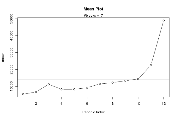
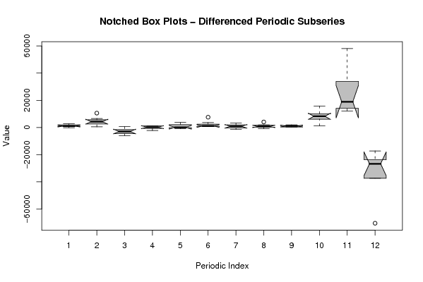
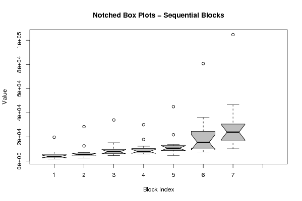
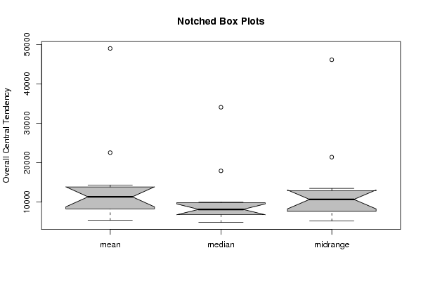
| Title produced by software | Mean Plot | ||||||||||||||||||||
| Date of computation | Sat, 06 Jun 2009 08:25:03 -0600 | ||||||||||||||||||||
| Cite this page as follows | Statistical Computations at FreeStatistics.org, Office for Research Development and Education, URL https://freestatistics.org/blog/index.php?v=date/2009/Jun/06/t1244298327qvez5ihb4k8o5hn.htm/, Retrieved Sun, 28 Apr 2024 23:52:03 +0000 | ||||||||||||||||||||
| Statistical Computations at FreeStatistics.org, Office for Research Development and Education, URL https://freestatistics.org/blog/index.php?pk=42008, Retrieved Sun, 28 Apr 2024 23:52:03 +0000 | |||||||||||||||||||||
| QR Codes: | |||||||||||||||||||||
|
| |||||||||||||||||||||
| Original text written by user: | |||||||||||||||||||||
| IsPrivate? | No (this computation is public) | ||||||||||||||||||||
| User-defined keywords | |||||||||||||||||||||
| Estimated Impact | 154 | ||||||||||||||||||||
Tree of Dependent Computations | |||||||||||||||||||||
| Family? (F = Feedback message, R = changed R code, M = changed R Module, P = changed Parameters, D = changed Data) | |||||||||||||||||||||
| - [Mean Plot] [Opdracht 6 oefeni...] [2009-04-30 17:29:26] [74be16979710d4c4e7c6647856088456] - D [Mean Plot] [Duncan Huysmans O...] [2009-06-05 14:13:53] [74be16979710d4c4e7c6647856088456] - P [Mean Plot] [] [2009-06-06 14:25:03] [d41d8cd98f00b204e9800998ecf8427e] [Current] | |||||||||||||||||||||
| Feedback Forum | |||||||||||||||||||||
Post a new message | |||||||||||||||||||||
Dataset | |||||||||||||||||||||
| Dataseries X: | |||||||||||||||||||||
1664.81 2397.53 2840.71 3547.29 3752.96 3714.74 4349.61 3566.34 5021.82 6423.48 7600.60 19756.21 2499.81 5198.24 7225.14 4806.03 5900.88 4951.34 6179.12 4752.15 5496.43 5835.10 12600.08 28541.72 4717.02 5702.63 9957.58 5304.78 6492.43 6630.80 7349.62 8176.62 8573.17 9690.50 15151.84 34061.01 5921.10 5814.58 12421.25 6369.77 7609.12 7224.75 8121.22 7979.25 8093.06 8476.70 17914.66 30114.41 4826.64 6470.23 9638.77 8821.17 8722.37 10209.48 11276.55 12552.22 11637.39 13606.89 21822.11 45060.69 7615.03 9849.69 14558.40 11587.33 9332.56 13082.09 16732.78 19888.61 23933.38 25391.35 36024.80 80721.71 10243.24 11266.88 21826.84 17357.33 15997.79 18601.53 26155.15 28586.52 30505.41 30821.33 46634.38 104660.67 | |||||||||||||||||||||
Tables (Output of Computation) | |||||||||||||||||||||
| |||||||||||||||||||||
Figures (Output of Computation) | |||||||||||||||||||||
Input Parameters & R Code | |||||||||||||||||||||
| Parameters (Session): | |||||||||||||||||||||
| par1 = 12 ; | |||||||||||||||||||||
| Parameters (R input): | |||||||||||||||||||||
| par1 = 12 ; | |||||||||||||||||||||
| R code (references can be found in the software module): | |||||||||||||||||||||
par1 <- as.numeric(par1) | |||||||||||||||||||||