Free Statistics
of Irreproducible Research!
Description of Statistical Computation | |||||||||||||||||||||
|---|---|---|---|---|---|---|---|---|---|---|---|---|---|---|---|---|---|---|---|---|---|
| Author's title | |||||||||||||||||||||
| Author | *Unverified author* | ||||||||||||||||||||
| R Software Module | rwasp_meanplot.wasp | ||||||||||||||||||||
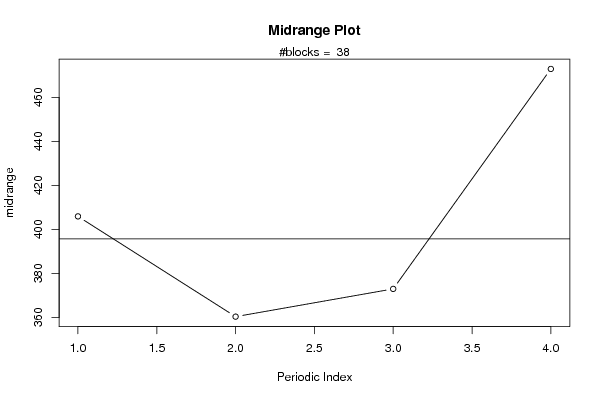
| Title produced by software | Mean Plot | ||||||||||||||||||||
| Date of computation | Mon, 26 Jan 2009 10:50:35 -0700 | ||||||||||||||||||||
| Cite this page as follows | Statistical Computations at FreeStatistics.org, Office for Research Development and Education, URL https://freestatistics.org/blog/index.php?v=date/2009/Jan/26/t1232992302efpdyifuor24oxs.htm/, Retrieved Sun, 05 May 2024 16:37:30 +0000 | ||||||||||||||||||||
| Statistical Computations at FreeStatistics.org, Office for Research Development and Education, URL https://freestatistics.org/blog/index.php?pk=36962, Retrieved Sun, 05 May 2024 16:37:30 +0000 | |||||||||||||||||||||
| QR Codes: | |||||||||||||||||||||
|
| |||||||||||||||||||||
| Original text written by user: | |||||||||||||||||||||
| IsPrivate? | No (this computation is public) | ||||||||||||||||||||
| User-defined keywords | |||||||||||||||||||||
| Estimated Impact | 197 | ||||||||||||||||||||
Tree of Dependent Computations | |||||||||||||||||||||
| Family? (F = Feedback message, R = changed R code, M = changed R Module, P = changed Parameters, D = changed Data) | |||||||||||||||||||||
| - [Mean Plot] [ Bierproductie in...] [2008-12-04 18:35:59] [73702d50a449ca9a9e8052b5a190ceb8] - PD [Mean Plot] [Robbe Leys_2MAR03...] [2009-01-26 17:50:35] [d41d8cd98f00b204e9800998ecf8427e] [Current] | |||||||||||||||||||||
| Feedback Forum | |||||||||||||||||||||
Post a new message | |||||||||||||||||||||
Dataset | |||||||||||||||||||||
| Dataseries X: | |||||||||||||||||||||
284.4 212.8 226.9 308.4 262 227.9 236.1 320.4 271.9 232.8 237 313.4 261.4 226.8 249.9 314.3 286.1 226.5 260.4 311.4 294.7 232.6 257.2 339.2 279.1 249.8 269.8 345.7 293.8 254.7 277.5 363.4 313.4 272.8 300.1 369.5 330.8 287.8 305.9 386.1 335.2 288 308.3 402.3 352.8 316.1 324.9 404.8 393 318.9 327 442.3 383.1 331.6 361.4 445.9 386.6 357.2 373.6 466.2 409.6 369.8 378.6 487 419.2 376.7 392.8 506.1 458.4 387.4 426.9 565 464.8 444.5 449.5 556.1 499.6 451.9 434.9 553.8 510 432.9 453.2 547.6 485.8 452.6 456.6 565.7 514.8 464.3 430.9 588.3 503.1 442.6 448 554.5 504.5 427.3 473.1 526.2 547.5 440.2 468.7 574.5 492.6 432.6 479.8 575.7 474.6 405.3 434.6 535.1 452.6 429.5 417.2 551.8 464 416.6 422.9 553.6 458.6 427.6 429.2 534.2 481.7 416 440.2 538.7 473.8 439.9 446.8 597.5 467.2 439.4 447.4 568.5 485.9 442.1 430.5 600 464.5 423.6 437 574 443 410 420 532 432 420 411 512 | |||||||||||||||||||||
Tables (Output of Computation) | |||||||||||||||||||||
| |||||||||||||||||||||
Figures (Output of Computation) | |||||||||||||||||||||
Input Parameters & R Code | |||||||||||||||||||||
| Parameters (Session): | |||||||||||||||||||||
| par1 = 4 ; | |||||||||||||||||||||
| Parameters (R input): | |||||||||||||||||||||
| par1 = 4 ; | |||||||||||||||||||||
| R code (references can be found in the software module): | |||||||||||||||||||||
par1 <- as.numeric(par1) | |||||||||||||||||||||