Free Statistics
of Irreproducible Research!
Description of Statistical Computation | |||||||||||||||||||||
|---|---|---|---|---|---|---|---|---|---|---|---|---|---|---|---|---|---|---|---|---|---|
| Author's title | |||||||||||||||||||||
| Author | *Unverified author* | ||||||||||||||||||||
| R Software Module | rwasp_sdplot.wasp | ||||||||||||||||||||
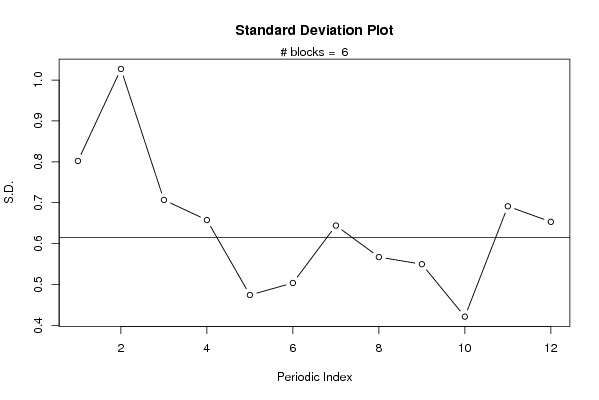
| Title produced by software | Standard Deviation Plot | ||||||||||||||||||||
| Date of computation | Sat, 10 Jan 2009 09:18:03 -0700 | ||||||||||||||||||||
| Cite this page as follows | Statistical Computations at FreeStatistics.org, Office for Research Development and Education, URL https://freestatistics.org/blog/index.php?v=date/2009/Jan/10/t1231604369xne77gh3nkyb3ef.htm/, Retrieved Mon, 29 Apr 2024 23:44:30 +0000 | ||||||||||||||||||||
| Statistical Computations at FreeStatistics.org, Office for Research Development and Education, URL https://freestatistics.org/blog/index.php?pk=36858, Retrieved Mon, 29 Apr 2024 23:44:30 +0000 | |||||||||||||||||||||
| QR Codes: | |||||||||||||||||||||
|
| |||||||||||||||||||||
| Original text written by user: | |||||||||||||||||||||
| IsPrivate? | No (this computation is public) | ||||||||||||||||||||
| User-defined keywords | |||||||||||||||||||||
| Estimated Impact | 225 | ||||||||||||||||||||
Tree of Dependent Computations | |||||||||||||||||||||
| Family? (F = Feedback message, R = changed R code, M = changed R Module, P = changed Parameters, D = changed Data) | |||||||||||||||||||||
| - [Standard Deviation Plot] [Opgave8 oefening ...] [2009-01-10 16:18:03] [d41d8cd98f00b204e9800998ecf8427e] [Current] - RM D [Standard Deviation-Mean Plot] [Opgave8 oefening ...] [2009-01-10 16:59:16] [74be16979710d4c4e7c6647856088456] | |||||||||||||||||||||
| Feedback Forum | |||||||||||||||||||||
Post a new message | |||||||||||||||||||||
Dataset | |||||||||||||||||||||
| Dataseries X: | |||||||||||||||||||||
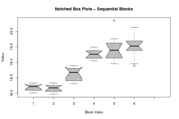
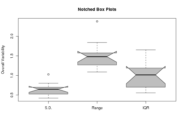
18,33 18,22 18,21 18,06 18,26 18,21 18,05 18,25 18,27 18,28 18,13 18,01 18,02 17,97 18,06 18,08 18,23 18,06 18,23 18,17 18,27 18,33 18,18 18,29 18,33 18,31 18,44 18,63 18,37 18,59 18,72 18,75 18,87 18,83 18,89 18,78 19,27 19,19 19,43 19,36 19,39 19,07 19,31 19,19 19,06 19,05 19,49 19,25 19,76 20,35 19,61 19,33 18,95 18,97 19,28 19,41 18,99 19,37 19,63 19,53 19,86 20,13 19,47 19,49 18,95 19,33 19,65 19,44 19,73 18,89 19,56 19,56 | |||||||||||||||||||||
Tables (Output of Computation) | |||||||||||||||||||||
| |||||||||||||||||||||
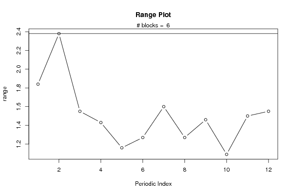
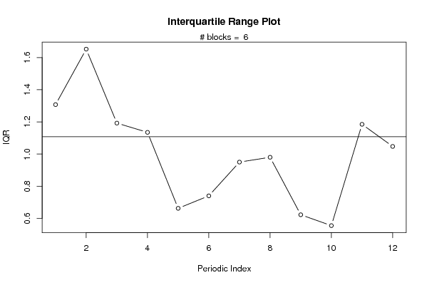
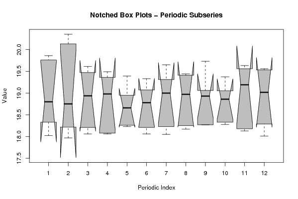
Figures (Output of Computation) | |||||||||||||||||||||
Input Parameters & R Code | |||||||||||||||||||||
| Parameters (Session): | |||||||||||||||||||||
| par1 = 12 ; | |||||||||||||||||||||
| Parameters (R input): | |||||||||||||||||||||
| par1 = 12 ; | |||||||||||||||||||||
| R code (references can be found in the software module): | |||||||||||||||||||||
par1 <- as.numeric(par1) | |||||||||||||||||||||