Free Statistics
of Irreproducible Research!
Description of Statistical Computation | |||||||||||||||||||||||||||||||||||||||||||||||||||||
|---|---|---|---|---|---|---|---|---|---|---|---|---|---|---|---|---|---|---|---|---|---|---|---|---|---|---|---|---|---|---|---|---|---|---|---|---|---|---|---|---|---|---|---|---|---|---|---|---|---|---|---|---|---|
| Author's title | |||||||||||||||||||||||||||||||||||||||||||||||||||||
| Author | *The author of this computation has been verified* | ||||||||||||||||||||||||||||||||||||||||||||||||||||
| R Software Module | rwasp_edauni.wasp | ||||||||||||||||||||||||||||||||||||||||||||||||||||
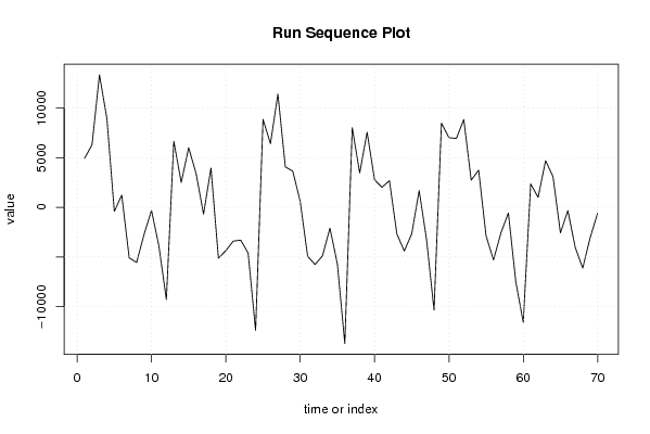
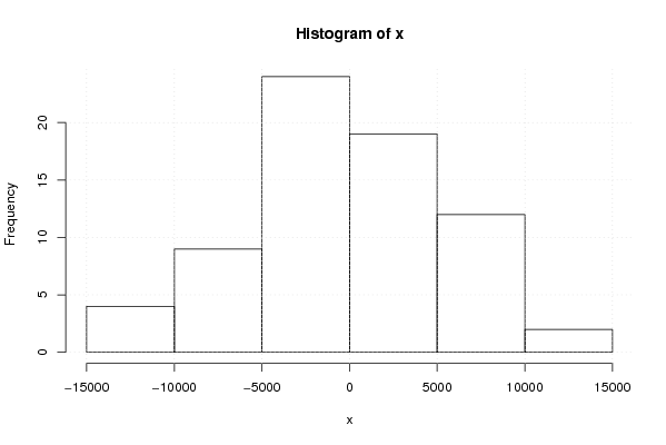
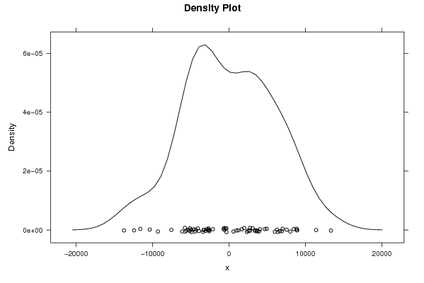
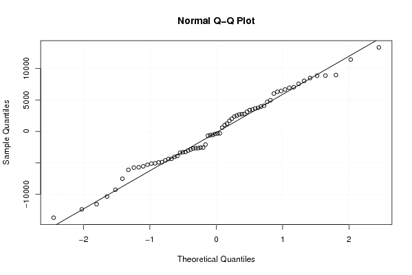
| Title produced by software | Univariate Explorative Data Analysis | ||||||||||||||||||||||||||||||||||||||||||||||||||||
| Date of computation | Wed, 30 Dec 2009 13:11:28 -0700 | ||||||||||||||||||||||||||||||||||||||||||||||||||||
| Cite this page as follows | Statistical Computations at FreeStatistics.org, Office for Research Development and Education, URL https://freestatistics.org/blog/index.php?v=date/2009/Dec/30/t1262203939uon4wug8rv9gskh.htm/, Retrieved Mon, 29 Apr 2024 03:00:46 +0000 | ||||||||||||||||||||||||||||||||||||||||||||||||||||
| Statistical Computations at FreeStatistics.org, Office for Research Development and Education, URL https://freestatistics.org/blog/index.php?pk=71367, Retrieved Mon, 29 Apr 2024 03:00:46 +0000 | |||||||||||||||||||||||||||||||||||||||||||||||||||||
| QR Codes: | |||||||||||||||||||||||||||||||||||||||||||||||||||||
|
| |||||||||||||||||||||||||||||||||||||||||||||||||||||
| Original text written by user: | |||||||||||||||||||||||||||||||||||||||||||||||||||||
| IsPrivate? | No (this computation is public) | ||||||||||||||||||||||||||||||||||||||||||||||||||||
| User-defined keywords | |||||||||||||||||||||||||||||||||||||||||||||||||||||
| Estimated Impact | 121 | ||||||||||||||||||||||||||||||||||||||||||||||||||||
Tree of Dependent Computations | |||||||||||||||||||||||||||||||||||||||||||||||||||||
| Family? (F = Feedback message, R = changed R code, M = changed R Module, P = changed Parameters, D = changed Data) | |||||||||||||||||||||||||||||||||||||||||||||||||||||
| - [Univariate Explorative Data Analysis] [] [2009-12-29 09:27:58] [d2d412c7f4d35ffbf5ee5ee89db327d4] - D [Univariate Explorative Data Analysis] [] [2009-12-30 14:10:39] [d2d412c7f4d35ffbf5ee5ee89db327d4] - D [Univariate Explorative Data Analysis] [] [2009-12-30 20:11:28] [f6a332ba2d530c028d935c5a5bbb53af] [Current] - D [Univariate Explorative Data Analysis] [] [2009-12-30 20:14:40] [d2d412c7f4d35ffbf5ee5ee89db327d4] | |||||||||||||||||||||||||||||||||||||||||||||||||||||
| Feedback Forum | |||||||||||||||||||||||||||||||||||||||||||||||||||||
Post a new message | |||||||||||||||||||||||||||||||||||||||||||||||||||||
Dataset | |||||||||||||||||||||||||||||||||||||||||||||||||||||
| Dataseries X: | |||||||||||||||||||||||||||||||||||||||||||||||||||||
4930,63 6284,63 13339,63 8935,63 -419,37 1220,63 -5094,37 -5561,37 -2732,37 -316,37 -3929,37 -9291,37 6644,63 2492,63 5997,63 3383,63 -693,37 3945,63 -5128,37 -4368,37 -3414,37 -3313,37 -4619,37 -12400,37 8857,63 6407,63 11407,63 4066,63 3637,63 592,63 -4941,37 -5770,37 -4893,37 -2103,37 -5716,37 -13731,37 8025,63 3452,63 7552,63 2760,63 2001,63 2679,63 -2680,37 -4410,37 -2674,37 1677,63 -3284,37 -10360,37 8467,63 7012,63 6920,63 8835,63 2727,63 3736,63 -2893,37 -5309,37 -2578,37 -580,37 -7526,37 -11589,37 2348,63 991,63 4687,63 3096,63 -2582,37 -339,37 -4070,37 -6127,37 -3062,37 -613,37 | |||||||||||||||||||||||||||||||||||||||||||||||||||||
Tables (Output of Computation) | |||||||||||||||||||||||||||||||||||||||||||||||||||||
| |||||||||||||||||||||||||||||||||||||||||||||||||||||
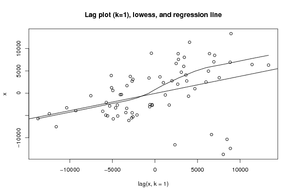
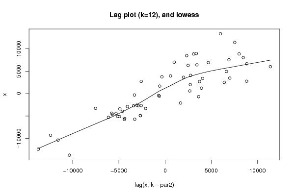
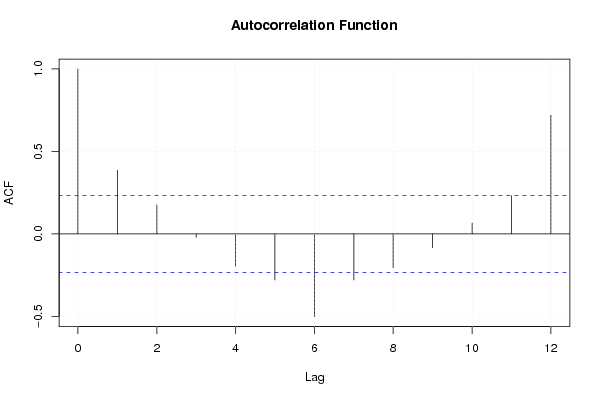
Figures (Output of Computation) | |||||||||||||||||||||||||||||||||||||||||||||||||||||
Input Parameters & R Code | |||||||||||||||||||||||||||||||||||||||||||||||||||||
| Parameters (Session): | |||||||||||||||||||||||||||||||||||||||||||||||||||||
| par1 = 0 ; par2 = 0 ; | |||||||||||||||||||||||||||||||||||||||||||||||||||||
| Parameters (R input): | |||||||||||||||||||||||||||||||||||||||||||||||||||||
| par1 = 0 ; par2 = 12 ; | |||||||||||||||||||||||||||||||||||||||||||||||||||||
| R code (references can be found in the software module): | |||||||||||||||||||||||||||||||||||||||||||||||||||||
par1 <- as.numeric(par1) | |||||||||||||||||||||||||||||||||||||||||||||||||||||