Repository of Reproducible Computations

Free Statistics

of Irreproducible Research!

Author's title

Author

*The author of this computation has been verified*

R Software Module

rwasp_arimaforecasting.wasp

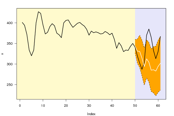
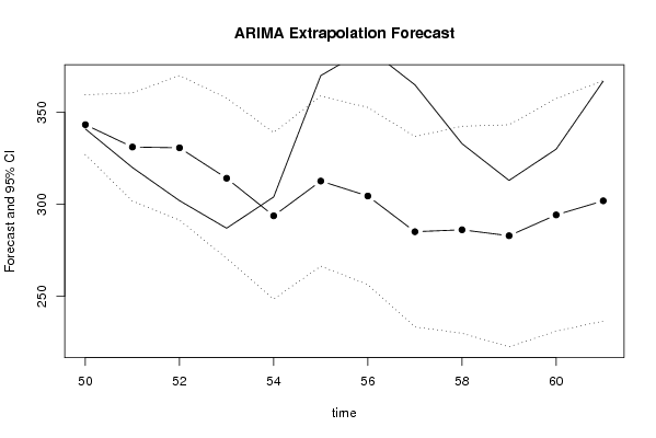
Title produced by software

ARIMA Forecasting

Date of computation

Wed, 30 Dec 2009 08:31:43 -0700

Cite this page as follows

Statistical Computations at FreeStatistics.org, Office for Research Development and Education, URL https://freestatistics.org/blog/index.php?v=date/2009/Dec/30/t1262187162dbed2phb4iclc31.htm/, Retrieved Mon, 29 Apr 2024 00:14:40 +0000

Statistical Computations at FreeStatistics.org, Office for Research Development and Education, URL https://freestatistics.org/blog/index.php?pk=71312, Retrieved Mon, 29 Apr 2024 00:14:40 +0000

QR Codes:

Paste this QR Code to cite your computation.

Original text written by user:

IsPrivate?

No (this computation is public)

User-defined keywords

Estimated Impact

145

Family? (F = Feedback message, R = changed R code, M = changed R Module, P = changed Parameters, D = changed Data)

-     [ARIMA Backward Selection] [arima backward se...] [2008-12-17 10:56:10] [11edab5c4db3615abbf782b1c6e7cacf]
- RMPD  [Central Tendency] [central tendency ...] [2008-12-23 10:31:31] [74be16979710d4c4e7c6647856088456]
- RMPD      [ARIMA Forecasting] [paper arima forec...] [2009-12-30 15:31:43] [1b03feaac1d41902024770a37504c07f] [Current]
- RMPD        [Multiple Regression] [paper multiple re...] [2009-12-30 16:08:31] [db72903d7941c8279d5ce0e4e873d517] 
- RMPD        [Multiple Regression] [paper multiple re...] [2009-12-30 16:26:00] [db72903d7941c8279d5ce0e4e873d517] 
- RMPD        [Multiple Regression] [paper multiple re...] [2009-12-30 16:37:41] [db72903d7941c8279d5ce0e4e873d517] 
- RMPD        [(Partial) Autocorrelation Function] [paper pacf export] [2009-12-30 16:59:53] [fd59abe368d8219a006d49608e51987e] 
- RMPD        [ARIMA Backward Selection] [paper arima backw...] [2009-12-30 17:31:23] [fd59abe368d8219a006d49608e51987e] 
- RMPD        [Central Tendency] [paper robustnessc...] [2009-12-30 17:38:16] [fd59abe368d8219a006d49608e51987e] 
-   PD        [ARIMA Forecasting] [paper arima forec...] [2009-12-30 18:07:08] [fd59abe368d8219a006d49608e51987e] 

Feedback Forum

Post a new message

Dataseries X:

Download CSV

Histogram

Boxplots

Summary of computational transaction
Raw Input	view raw input (R code)
Raw Output	view raw output of R engine
Computing time	3 seconds
R Server	'Gwilym Jenkins' @ 72.249.127.135

\begin{tabular}{lllllllll}
\hline
Summary of computational transaction \tabularnewline
Raw Input & view raw input (R code)  \tabularnewline
Raw Output & view raw output of R engine  \tabularnewline
Computing time & 3 seconds \tabularnewline
R Server & 'Gwilym Jenkins' @ 72.249.127.135 \tabularnewline
\hline
\end{tabular}
%Source: https://freestatistics.org/blog/index.php?pk=71312&T=0

[TABLE]
[ROW][C]Summary of computational transaction[/C][/ROW]
[ROW][C]Raw Input[/C][C]view raw input (R code) [/C][/ROW]
[ROW][C]Raw Output[/C][C]view raw output of R engine [/C][/ROW]
[ROW][C]Computing time[/C][C]3 seconds[/C][/ROW]
[ROW][C]R Server[/C][C]'Gwilym Jenkins' @ 72.249.127.135[/C][/ROW]
[/TABLE]
Source: https://freestatistics.org/blog/index.php?pk=71312&T=0

Globally Unique Identifier (entire table): ba.freestatistics.org/blog/index.php?pk=71312&T=0

As an alternative you can also use a QR Code:

The GUIDs for individual cells are displayed in the table below:

Summary of computational transaction
Raw Input	view raw input (R code)
Raw Output	view raw output of R engine
Computing time	3 seconds
R Server	'Gwilym Jenkins' @ 72.249.127.135

Univariate ARIMA Extrapolation Forecast
time	Y[t]	F[t]	95% LB	95% UB	p-value(H0: Y[t] = F[t])	P(F[t]>Y[t-1])	P(F[t]>Y[t-s])	P(F[t]>Y[49])
37	379	-	-	-	-	-	-	-
38	376	-	-	-	-	-	-	-
39	371	-	-	-	-	-	-	-
40	375	-	-	-	-	-	-	-
41	360	-	-	-	-	-	-	-
42	338	-	-	-	-	-	-	-
43	352	-	-	-	-	-	-	-
44	344	-	-	-	-	-	-	-
45	330	-	-	-	-	-	-	-
46	334	-	-	-	-	-	-	-
47	333	-	-	-	-	-	-	-
48	343	-	-	-	-	-	-	-
49	350	-	-	-	-	-	-	-
50	341	343.3155	327.0106	359.6204	0.3904	0.2108	0	0.2108
51	320	331.1696	301.7381	360.6012	0.2285	0.2563	0.004	0.1049
52	302	330.736	291.406	370.0659	0.0761	0.7037	0.0137	0.1685
53	287	314.1852	270.5636	357.8068	0.111	0.708	0.0198	0.0538
54	304	293.7576	248.5113	339.004	0.3286	0.6151	0.0277	0.0074
55	370	312.6566	266.3828	358.9305	0.0076	0.6431	0.0478	0.0569
56	385	304.5286	256.3571	352.7	5e-04	0.0039	0.0541	0.0321
57	365	285.107	233.3696	336.8444	0.0012	1e-04	0.0445	0.007
58	333	286.1605	229.8496	342.4715	0.0515	0.003	0.0479	0.0131
59	313	282.9175	222.5625	343.2725	0.1643	0.0519	0.0519	0.0147
60	330	294.2509	231.0018	357.4999	0.134	0.2806	0.0654	0.042
61	367	301.9051	236.5259	367.2843	0.0255	0.1998	0.0747	0.0747

\begin{tabular}{lllllllll}
\hline
Univariate ARIMA Extrapolation Forecast \tabularnewline
time & Y[t] & F[t] & 95% LB & 95% UB & p-value(H0: Y[t] = F[t]) & P(F[t]>Y[t-1]) & P(F[t]>Y[t-s]) & P(F[t]>Y[49]) \tabularnewline
37 & 379 & - & - & - & - & - & - & - \tabularnewline
38 & 376 & - & - & - & - & - & - & - \tabularnewline
39 & 371 & - & - & - & - & - & - & - \tabularnewline
40 & 375 & - & - & - & - & - & - & - \tabularnewline
41 & 360 & - & - & - & - & - & - & - \tabularnewline
42 & 338 & - & - & - & - & - & - & - \tabularnewline
43 & 352 & - & - & - & - & - & - & - \tabularnewline
44 & 344 & - & - & - & - & - & - & - \tabularnewline
45 & 330 & - & - & - & - & - & - & - \tabularnewline
46 & 334 & - & - & - & - & - & - & - \tabularnewline
47 & 333 & - & - & - & - & - & - & - \tabularnewline
48 & 343 & - & - & - & - & - & - & - \tabularnewline
49 & 350 & - & - & - & - & - & - & - \tabularnewline
50 & 341 & 343.3155 & 327.0106 & 359.6204 & 0.3904 & 0.2108 & 0 & 0.2108 \tabularnewline
51 & 320 & 331.1696 & 301.7381 & 360.6012 & 0.2285 & 0.2563 & 0.004 & 0.1049 \tabularnewline
52 & 302 & 330.736 & 291.406 & 370.0659 & 0.0761 & 0.7037 & 0.0137 & 0.1685 \tabularnewline
53 & 287 & 314.1852 & 270.5636 & 357.8068 & 0.111 & 0.708 & 0.0198 & 0.0538 \tabularnewline
54 & 304 & 293.7576 & 248.5113 & 339.004 & 0.3286 & 0.6151 & 0.0277 & 0.0074 \tabularnewline
55 & 370 & 312.6566 & 266.3828 & 358.9305 & 0.0076 & 0.6431 & 0.0478 & 0.0569 \tabularnewline
56 & 385 & 304.5286 & 256.3571 & 352.7 & 5e-04 & 0.0039 & 0.0541 & 0.0321 \tabularnewline
57 & 365 & 285.107 & 233.3696 & 336.8444 & 0.0012 & 1e-04 & 0.0445 & 0.007 \tabularnewline
58 & 333 & 286.1605 & 229.8496 & 342.4715 & 0.0515 & 0.003 & 0.0479 & 0.0131 \tabularnewline
59 & 313 & 282.9175 & 222.5625 & 343.2725 & 0.1643 & 0.0519 & 0.0519 & 0.0147 \tabularnewline
60 & 330 & 294.2509 & 231.0018 & 357.4999 & 0.134 & 0.2806 & 0.0654 & 0.042 \tabularnewline
61 & 367 & 301.9051 & 236.5259 & 367.2843 & 0.0255 & 0.1998 & 0.0747 & 0.0747 \tabularnewline
\hline
\end{tabular}
%Source: https://freestatistics.org/blog/index.php?pk=71312&T=1

[TABLE]
[ROW][C]Univariate ARIMA Extrapolation Forecast[/C][/ROW]
[ROW][C]time[/C][C]Y[t][/C][C]F[t][/C][C]95% LB[/C][C]95% UB[/C][C]p-value(H0: Y[t] = F[t])[/C][C]P(F[t]>Y[t-1])[/C][C]P(F[t]>Y[t-s])[/C][C]P(F[t]>Y[49])[/C][/ROW]
[ROW][C]37[/C][C]379[/C][C]-[/C][C]-[/C][C]-[/C][C]-[/C][C]-[/C][C]-[/C][C]-[/C][/ROW]
[ROW][C]38[/C][C]376[/C][C]-[/C][C]-[/C][C]-[/C][C]-[/C][C]-[/C][C]-[/C][C]-[/C][/ROW]
[ROW][C]39[/C][C]371[/C][C]-[/C][C]-[/C][C]-[/C][C]-[/C][C]-[/C][C]-[/C][C]-[/C][/ROW]
[ROW][C]40[/C][C]375[/C][C]-[/C][C]-[/C][C]-[/C][C]-[/C][C]-[/C][C]-[/C][C]-[/C][/ROW]
[ROW][C]41[/C][C]360[/C][C]-[/C][C]-[/C][C]-[/C][C]-[/C][C]-[/C][C]-[/C][C]-[/C][/ROW]
[ROW][C]42[/C][C]338[/C][C]-[/C][C]-[/C][C]-[/C][C]-[/C][C]-[/C][C]-[/C][C]-[/C][/ROW]
[ROW][C]43[/C][C]352[/C][C]-[/C][C]-[/C][C]-[/C][C]-[/C][C]-[/C][C]-[/C][C]-[/C][/ROW]
[ROW][C]44[/C][C]344[/C][C]-[/C][C]-[/C][C]-[/C][C]-[/C][C]-[/C][C]-[/C][C]-[/C][/ROW]
[ROW][C]45[/C][C]330[/C][C]-[/C][C]-[/C][C]-[/C][C]-[/C][C]-[/C][C]-[/C][C]-[/C][/ROW]
[ROW][C]46[/C][C]334[/C][C]-[/C][C]-[/C][C]-[/C][C]-[/C][C]-[/C][C]-[/C][C]-[/C][/ROW]
[ROW][C]47[/C][C]333[/C][C]-[/C][C]-[/C][C]-[/C][C]-[/C][C]-[/C][C]-[/C][C]-[/C][/ROW]
[ROW][C]48[/C][C]343[/C][C]-[/C][C]-[/C][C]-[/C][C]-[/C][C]-[/C][C]-[/C][C]-[/C][/ROW]
[ROW][C]49[/C][C]350[/C][C]-[/C][C]-[/C][C]-[/C][C]-[/C][C]-[/C][C]-[/C][C]-[/C][/ROW]
[ROW][C]50[/C][C]341[/C][C]343.3155[/C][C]327.0106[/C][C]359.6204[/C][C]0.3904[/C][C]0.2108[/C][C]0[/C][C]0.2108[/C][/ROW]
[ROW][C]51[/C][C]320[/C][C]331.1696[/C][C]301.7381[/C][C]360.6012[/C][C]0.2285[/C][C]0.2563[/C][C]0.004[/C][C]0.1049[/C][/ROW]
[ROW][C]52[/C][C]302[/C][C]330.736[/C][C]291.406[/C][C]370.0659[/C][C]0.0761[/C][C]0.7037[/C][C]0.0137[/C][C]0.1685[/C][/ROW]
[ROW][C]53[/C][C]287[/C][C]314.1852[/C][C]270.5636[/C][C]357.8068[/C][C]0.111[/C][C]0.708[/C][C]0.0198[/C][C]0.0538[/C][/ROW]
[ROW][C]54[/C][C]304[/C][C]293.7576[/C][C]248.5113[/C][C]339.004[/C][C]0.3286[/C][C]0.6151[/C][C]0.0277[/C][C]0.0074[/C][/ROW]
[ROW][C]55[/C][C]370[/C][C]312.6566[/C][C]266.3828[/C][C]358.9305[/C][C]0.0076[/C][C]0.6431[/C][C]0.0478[/C][C]0.0569[/C][/ROW]
[ROW][C]56[/C][C]385[/C][C]304.5286[/C][C]256.3571[/C][C]352.7[/C][C]5e-04[/C][C]0.0039[/C][C]0.0541[/C][C]0.0321[/C][/ROW]
[ROW][C]57[/C][C]365[/C][C]285.107[/C][C]233.3696[/C][C]336.8444[/C][C]0.0012[/C][C]1e-04[/C][C]0.0445[/C][C]0.007[/C][/ROW]
[ROW][C]58[/C][C]333[/C][C]286.1605[/C][C]229.8496[/C][C]342.4715[/C][C]0.0515[/C][C]0.003[/C][C]0.0479[/C][C]0.0131[/C][/ROW]
[ROW][C]59[/C][C]313[/C][C]282.9175[/C][C]222.5625[/C][C]343.2725[/C][C]0.1643[/C][C]0.0519[/C][C]0.0519[/C][C]0.0147[/C][/ROW]
[ROW][C]60[/C][C]330[/C][C]294.2509[/C][C]231.0018[/C][C]357.4999[/C][C]0.134[/C][C]0.2806[/C][C]0.0654[/C][C]0.042[/C][/ROW]
[ROW][C]61[/C][C]367[/C][C]301.9051[/C][C]236.5259[/C][C]367.2843[/C][C]0.0255[/C][C]0.1998[/C][C]0.0747[/C][C]0.0747[/C][/ROW]
[/TABLE]
Source: https://freestatistics.org/blog/index.php?pk=71312&T=1

Globally Unique Identifier (entire table): ba.freestatistics.org/blog/index.php?pk=71312&T=1

As an alternative you can also use a QR Code:

The GUIDs for individual cells are displayed in the table below:

Univariate ARIMA Extrapolation Forecast
time	Y[t]	F[t]	95% LB	95% UB	p-value(H0: Y[t] = F[t])	P(F[t]>Y[t-1])	P(F[t]>Y[t-s])	P(F[t]>Y[49])
37	379	-	-	-	-	-	-	-
38	376	-	-	-	-	-	-	-
39	371	-	-	-	-	-	-	-
40	375	-	-	-	-	-	-	-
41	360	-	-	-	-	-	-	-
42	338	-	-	-	-	-	-	-
43	352	-	-	-	-	-	-	-
44	344	-	-	-	-	-	-	-
45	330	-	-	-	-	-	-	-
46	334	-	-	-	-	-	-	-
47	333	-	-	-	-	-	-	-
48	343	-	-	-	-	-	-	-
49	350	-	-	-	-	-	-	-
50	341	343.3155	327.0106	359.6204	0.3904	0.2108	0	0.2108
51	320	331.1696	301.7381	360.6012	0.2285	0.2563	0.004	0.1049
52	302	330.736	291.406	370.0659	0.0761	0.7037	0.0137	0.1685
53	287	314.1852	270.5636	357.8068	0.111	0.708	0.0198	0.0538
54	304	293.7576	248.5113	339.004	0.3286	0.6151	0.0277	0.0074
55	370	312.6566	266.3828	358.9305	0.0076	0.6431	0.0478	0.0569
56	385	304.5286	256.3571	352.7	5e-04	0.0039	0.0541	0.0321
57	365	285.107	233.3696	336.8444	0.0012	1e-04	0.0445	0.007
58	333	286.1605	229.8496	342.4715	0.0515	0.003	0.0479	0.0131
59	313	282.9175	222.5625	343.2725	0.1643	0.0519	0.0519	0.0147
60	330	294.2509	231.0018	357.4999	0.134	0.2806	0.0654	0.042
61	367	301.9051	236.5259	367.2843	0.0255	0.1998	0.0747	0.0747

Univariate ARIMA Extrapolation Forecast Performance
time	% S.E.	PE	MAPE	Sq.E	MSE	RMSE
50	0.0242	-0.0067	0	5.3615	0	0
51	0.0453	-0.0337	0.0202	124.7604	65.0609	8.066
52	0.0607	-0.0869	0.0425	825.757	318.6263	17.8501
53	0.0708	-0.0865	0.0535	739.0333	423.728	20.5847
54	0.0786	0.0349	0.0497	104.9062	359.9637	18.9727
55	0.0755	0.1834	0.072	3288.2625	848.0135	29.1207
56	0.0807	0.2642	0.0995	6475.6494	1651.9615	40.6443
57	0.0926	0.2802	0.1221	6382.8907	2243.3276	47.3638
58	0.1004	0.1637	0.1267	2193.9367	2237.8397	47.3058
59	0.1088	0.1063	0.1247	904.9587	2104.5516	45.8754
60	0.1097	0.1215	0.1244	1277.9992	2029.4105	45.049
61	0.1105	0.2156	0.132	4237.3425	2213.4048	47.0468

\begin{tabular}{lllllllll}
\hline
Univariate ARIMA Extrapolation Forecast Performance \tabularnewline
time & % S.E. & PE & MAPE & Sq.E & MSE & RMSE \tabularnewline
50 & 0.0242 & -0.0067 & 0 & 5.3615 & 0 & 0 \tabularnewline
51 & 0.0453 & -0.0337 & 0.0202 & 124.7604 & 65.0609 & 8.066 \tabularnewline
52 & 0.0607 & -0.0869 & 0.0425 & 825.757 & 318.6263 & 17.8501 \tabularnewline
53 & 0.0708 & -0.0865 & 0.0535 & 739.0333 & 423.728 & 20.5847 \tabularnewline
54 & 0.0786 & 0.0349 & 0.0497 & 104.9062 & 359.9637 & 18.9727 \tabularnewline
55 & 0.0755 & 0.1834 & 0.072 & 3288.2625 & 848.0135 & 29.1207 \tabularnewline
56 & 0.0807 & 0.2642 & 0.0995 & 6475.6494 & 1651.9615 & 40.6443 \tabularnewline
57 & 0.0926 & 0.2802 & 0.1221 & 6382.8907 & 2243.3276 & 47.3638 \tabularnewline
58 & 0.1004 & 0.1637 & 0.1267 & 2193.9367 & 2237.8397 & 47.3058 \tabularnewline
59 & 0.1088 & 0.1063 & 0.1247 & 904.9587 & 2104.5516 & 45.8754 \tabularnewline
60 & 0.1097 & 0.1215 & 0.1244 & 1277.9992 & 2029.4105 & 45.049 \tabularnewline
61 & 0.1105 & 0.2156 & 0.132 & 4237.3425 & 2213.4048 & 47.0468 \tabularnewline
\hline
\end{tabular}
%Source: https://freestatistics.org/blog/index.php?pk=71312&T=2

[TABLE]
[ROW][C]Univariate ARIMA Extrapolation Forecast Performance[/C][/ROW]
[ROW][C]time[/C][C]% S.E.[/C][C]PE[/C][C]MAPE[/C][C]Sq.E[/C][C]MSE[/C][C]RMSE[/C][/ROW]
[ROW][C]50[/C][C]0.0242[/C][C]-0.0067[/C][C]0[/C][C]5.3615[/C][C]0[/C][C]0[/C][/ROW]
[ROW][C]51[/C][C]0.0453[/C][C]-0.0337[/C][C]0.0202[/C][C]124.7604[/C][C]65.0609[/C][C]8.066[/C][/ROW]
[ROW][C]52[/C][C]0.0607[/C][C]-0.0869[/C][C]0.0425[/C][C]825.757[/C][C]318.6263[/C][C]17.8501[/C][/ROW]
[ROW][C]53[/C][C]0.0708[/C][C]-0.0865[/C][C]0.0535[/C][C]739.0333[/C][C]423.728[/C][C]20.5847[/C][/ROW]
[ROW][C]54[/C][C]0.0786[/C][C]0.0349[/C][C]0.0497[/C][C]104.9062[/C][C]359.9637[/C][C]18.9727[/C][/ROW]
[ROW][C]55[/C][C]0.0755[/C][C]0.1834[/C][C]0.072[/C][C]3288.2625[/C][C]848.0135[/C][C]29.1207[/C][/ROW]
[ROW][C]56[/C][C]0.0807[/C][C]0.2642[/C][C]0.0995[/C][C]6475.6494[/C][C]1651.9615[/C][C]40.6443[/C][/ROW]
[ROW][C]57[/C][C]0.0926[/C][C]0.2802[/C][C]0.1221[/C][C]6382.8907[/C][C]2243.3276[/C][C]47.3638[/C][/ROW]
[ROW][C]58[/C][C]0.1004[/C][C]0.1637[/C][C]0.1267[/C][C]2193.9367[/C][C]2237.8397[/C][C]47.3058[/C][/ROW]
[ROW][C]59[/C][C]0.1088[/C][C]0.1063[/C][C]0.1247[/C][C]904.9587[/C][C]2104.5516[/C][C]45.8754[/C][/ROW]
[ROW][C]60[/C][C]0.1097[/C][C]0.1215[/C][C]0.1244[/C][C]1277.9992[/C][C]2029.4105[/C][C]45.049[/C][/ROW]
[ROW][C]61[/C][C]0.1105[/C][C]0.2156[/C][C]0.132[/C][C]4237.3425[/C][C]2213.4048[/C][C]47.0468[/C][/ROW]
[/TABLE]
Source: https://freestatistics.org/blog/index.php?pk=71312&T=2

Globally Unique Identifier (entire table): ba.freestatistics.org/blog/index.php?pk=71312&T=2

As an alternative you can also use a QR Code:

The GUIDs for individual cells are displayed in the table below:

Univariate ARIMA Extrapolation Forecast Performance
time	% S.E.	PE	MAPE	Sq.E	MSE	RMSE
50	0.0242	-0.0067	0	5.3615	0	0
51	0.0453	-0.0337	0.0202	124.7604	65.0609	8.066
52	0.0607	-0.0869	0.0425	825.757	318.6263	17.8501
53	0.0708	-0.0865	0.0535	739.0333	423.728	20.5847
54	0.0786	0.0349	0.0497	104.9062	359.9637	18.9727
55	0.0755	0.1834	0.072	3288.2625	848.0135	29.1207
56	0.0807	0.2642	0.0995	6475.6494	1651.9615	40.6443
57	0.0926	0.2802	0.1221	6382.8907	2243.3276	47.3638
58	0.1004	0.1637	0.1267	2193.9367	2237.8397	47.3058
59	0.1088	0.1063	0.1247	904.9587	2104.5516	45.8754
60	0.1097	0.1215	0.1244	1277.9992	2029.4105	45.049
61	0.1105	0.2156	0.132	4237.3425	2213.4048	47.0468

Figure 1

PNG link

Postscript link

PDF link

Figure 2

PNG link

Postscript link

PDF link

Parameters (Session):

par1 = 12 ; par2 = 1 ; par3 = 2 ; par4 = 1 ; par5 = 12 ; par6 = 3 ; par7 = 1 ; par8 = 2 ; par9 = 0 ; par10 = FALSE ;

Parameters (R input):

par1 = 12 ; par2 = 1 ; par3 = 2 ; par4 = 1 ; par5 = 12 ; par6 = 3 ; par7 = 1 ; par8 = 2 ; par9 = 0 ; par10 = FALSE ;

R code (references can be found in the software module):

par1 <- as.numeric(par1) #cut off periods
par2 <- as.numeric(par2) #lambda
par3 <- as.numeric(par3) #degree of non-seasonal differencing
par4 <- as.numeric(par4) #degree of seasonal differencing
par5 <- as.numeric(par5) #seasonal period
par6 <- as.numeric(par6) #p
par7 <- as.numeric(par7) #q
par8 <- as.numeric(par8) #P
par9 <- as.numeric(par9) #Q
if (par10 == 'TRUE') par10 <- TRUE
if (par10 == 'FALSE') par10 <- FALSE
if (par2 == 0) x <- log(x)
if (par2 != 0) x <- x^par2
lx <- length(x)
first <- lx - 2*par1
nx <- lx - par1
nx1 <- nx + 1
fx <- lx - nx
if (fx < 1) {
fx <- par5
nx1 <- lx + fx - 1
first <- lx - 2*fx
}
first <- 1
if (fx < 3) fx <- round(lx/10,0)
(arima.out <- arima(x[1:nx], order=c(par6,par3,par7), seasonal=list(order=c(par8,par4,par9), period=par5), include.mean=par10, method='ML'))
(forecast <- predict(arima.out,par1))
(lb <- forecast$pred - 1.96 * forecast$se)
(ub <- forecast$pred + 1.96 * forecast$se)
if (par2 == 0) {
x <- exp(x)
forecast$pred <- exp(forecast$pred)
lb <- exp(lb)
ub <- exp(ub)
}
if (par2 != 0) {
x <- x^(1/par2)
forecast$pred <- forecast$pred^(1/par2)
lb <- lb^(1/par2)
ub <- ub^(1/par2)
}
if (par2 < 0) {
olb <- lb
lb <- ub
ub <- olb
}
(actandfor <- c(x[1:nx], forecast$pred))
(perc.se <- (ub-forecast$pred)/1.96/forecast$pred)
bitmap(file='test1.png')
opar <- par(mar=c(4,4,2,2),las=1)
ylim <- c( min(x[first:nx],lb), max(x[first:nx],ub))
plot(x,ylim=ylim,type='n',xlim=c(first,lx))
usr <- par('usr')
rect(usr[1],usr[3],nx+1,usr[4],border=NA,col='lemonchiffon')
rect(nx1,usr[3],usr[2],usr[4],border=NA,col='lavender')
abline(h= (-3:3)*2 , col ='gray', lty =3)
polygon( c(nx1:lx,lx:nx1), c(lb,rev(ub)), col = 'orange', lty=2,border=NA)
lines(nx1:lx, lb , lty=2)
lines(nx1:lx, ub , lty=2)
lines(x, lwd=2)
lines(nx1:lx, forecast$pred , lwd=2 , col ='white')
box()
par(opar)
dev.off()
prob.dec <- array(NA, dim=fx)
prob.sdec <- array(NA, dim=fx)
prob.ldec <- array(NA, dim=fx)
prob.pval <- array(NA, dim=fx)
perf.pe <- array(0, dim=fx)
perf.mape <- array(0, dim=fx)
perf.mape1 <- array(0, dim=fx)
perf.se <- array(0, dim=fx)
perf.mse <- array(0, dim=fx)
perf.mse1 <- array(0, dim=fx)
perf.rmse <- array(0, dim=fx)
for (i in 1:fx) {
locSD <- (ub[i] - forecast$pred[i]) / 1.96
perf.pe[i] = (x[nx+i] - forecast$pred[i]) / forecast$pred[i]
perf.se[i] = (x[nx+i] - forecast$pred[i])^2
prob.dec[i] = pnorm((x[nx+i-1] - forecast$pred[i]) / locSD)
prob.sdec[i] = pnorm((x[nx+i-par5] - forecast$pred[i]) / locSD)
prob.ldec[i] = pnorm((x[nx] - forecast$pred[i]) / locSD)
prob.pval[i] = pnorm(abs(x[nx+i] - forecast$pred[i]) / locSD)
}
perf.mape[1] = abs(perf.pe[1])
perf.mse[1] = abs(perf.se[1])
for (i in 2:fx) {
perf.mape[i] = perf.mape[i-1] + abs(perf.pe[i])
perf.mape1[i] = perf.mape[i] / i
perf.mse[i] = perf.mse[i-1] + perf.se[i]
perf.mse1[i] = perf.mse[i] / i
}
perf.rmse = sqrt(perf.mse1)
bitmap(file='test2.png')
plot(forecast$pred, pch=19, type='b',main='ARIMA Extrapolation Forecast', ylab='Forecast and 95% CI', xlab='time',ylim=c(min(lb),max(ub)))
dum <- forecast$pred
dum[1:par1] <- x[(nx+1):lx]
lines(dum, lty=1)
lines(ub,lty=3)
lines(lb,lty=3)
dev.off()
load(file='createtable')
a<-table.start()
a<-table.row.start(a)
a<-table.element(a,'Univariate ARIMA Extrapolation Forecast',9,TRUE)
a<-table.row.end(a)
a<-table.row.start(a)
a<-table.element(a,'time',1,header=TRUE)
a<-table.element(a,'Y[t]',1,header=TRUE)
a<-table.element(a,'F[t]',1,header=TRUE)
a<-table.element(a,'95% LB',1,header=TRUE)
a<-table.element(a,'95% UB',1,header=TRUE)
a<-table.element(a,'p-value
(H0: Y[t] = F[t])',1,header=TRUE)
a<-table.element(a,'P(F[t]>Y[t-1])',1,header=TRUE)
a<-table.element(a,'P(F[t]>Y[t-s])',1,header=TRUE)
mylab <- paste('P(F[t]>Y[',nx,sep='')
mylab <- paste(mylab,'])',sep='')
a<-table.element(a,mylab,1,header=TRUE)
a<-table.row.end(a)
for (i in (nx-par5):nx) {
a<-table.row.start(a)
a<-table.element(a,i,header=TRUE)
a<-table.element(a,x[i])
a<-table.element(a,'-')
a<-table.element(a,'-')
a<-table.element(a,'-')
a<-table.element(a,'-')
a<-table.element(a,'-')
a<-table.element(a,'-')
a<-table.element(a,'-')
a<-table.row.end(a)
}
for (i in 1:fx) {
a<-table.row.start(a)
a<-table.element(a,nx+i,header=TRUE)
a<-table.element(a,round(x[nx+i],4))
a<-table.element(a,round(forecast$pred[i],4))
a<-table.element(a,round(lb[i],4))
a<-table.element(a,round(ub[i],4))
a<-table.element(a,round((1-prob.pval[i]),4))
a<-table.element(a,round((1-prob.dec[i]),4))
a<-table.element(a,round((1-prob.sdec[i]),4))
a<-table.element(a,round((1-prob.ldec[i]),4))
a<-table.row.end(a)
}
a<-table.end(a)
table.save(a,file='mytable.tab')
a<-table.start()
a<-table.row.start(a)
a<-table.element(a,'Univariate ARIMA Extrapolation Forecast Performance',7,TRUE)
a<-table.row.end(a)
a<-table.row.start(a)
a<-table.element(a,'time',1,header=TRUE)
a<-table.element(a,'% S.E.',1,header=TRUE)
a<-table.element(a,'PE',1,header=TRUE)
a<-table.element(a,'MAPE',1,header=TRUE)
a<-table.element(a,'Sq.E',1,header=TRUE)
a<-table.element(a,'MSE',1,header=TRUE)
a<-table.element(a,'RMSE',1,header=TRUE)
a<-table.row.end(a)
for (i in 1:fx) {
a<-table.row.start(a)
a<-table.element(a,nx+i,header=TRUE)
a<-table.element(a,round(perc.se[i],4))
a<-table.element(a,round(perf.pe[i],4))
a<-table.element(a,round(perf.mape1[i],4))
a<-table.element(a,round(perf.se[i],4))
a<-table.element(a,round(perf.mse1[i],4))
a<-table.element(a,round(perf.rmse[i],4))
a<-table.row.end(a)
}
a<-table.end(a)
table.save(a,file='mytable1.tab')

Free Statistics

Description of Statistical Computation

Tree of Dependent Computations

Dataset

Tables (Output of Computation)

Figures (Output of Computation)

Input Parameters & R Code