Repository of Reproducible Computations

Free Statistics

of Irreproducible Research!

Author's title

Author

*The author of this computation has been verified*

R Software Module

rwasp_autocorrelation.wasp

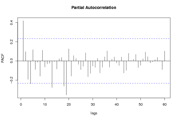
Title produced by software

(Partial) Autocorrelation Function

Date of computation

Wed, 30 Dec 2009 06:42:19 -0700

Cite this page as follows

Statistical Computations at FreeStatistics.org, Office for Research Development and Education, URL https://freestatistics.org/blog/index.php?v=date/2009/Dec/30/t1262180630ji4ihachn2px2em.htm/, Retrieved Mon, 29 Apr 2024 00:40:18 +0000

Statistical Computations at FreeStatistics.org, Office for Research Development and Education, URL https://freestatistics.org/blog/index.php?pk=71277, Retrieved Mon, 29 Apr 2024 00:40:18 +0000

QR Codes:

Paste this QR Code to cite your computation.

Original text written by user:

IsPrivate?

No (this computation is public)

User-defined keywords

Estimated Impact

151

Family? (F = Feedback message, R = changed R code, M = changed R Module, P = changed Parameters, D = changed Data)

-     [Univariate Data Series] [De Belgische uitv...] [2009-10-13 01:35:54] [df6326eec97a6ca984a853b142930499]
- RMPD  [Univariate Data Series] [ws8] [2009-11-27 12:04:12] [acdebb2ecda2ddb208f4e14f4a68b9e7]
-   PD    [Univariate Data Series] [consumptiekrediet] [2009-12-04 10:09:44] [acdebb2ecda2ddb208f4e14f4a68b9e7]
-   PD      [Univariate Data Series] [Verkoopprijs per ...] [2009-12-20 19:05:51] [acdebb2ecda2ddb208f4e14f4a68b9e7]
- RMPD          [(Partial) Autocorrelation Function] [Autocorrelatiefun...] [2009-12-30 13:42:19] [b243db81ea3e1f02fb3382887fb0f701] [Current]
-   P             [(Partial) Autocorrelation Function] [Autocorrelatiefun...] [2009-12-31 10:14:57] [acdebb2ecda2ddb208f4e14f4a68b9e7] 

Feedback Forum

Post a new message

Dataseries X:

Download CSV

Histogram

Boxplots

Summary of computational transaction
Raw Input	view raw input (R code)
Raw Output	view raw output of R engine
Computing time	2 seconds
R Server	'Gwilym Jenkins' @ 72.249.127.135

\begin{tabular}{lllllllll}
\hline
Summary of computational transaction \tabularnewline
Raw Input & view raw input (R code)  \tabularnewline
Raw Output & view raw output of R engine  \tabularnewline
Computing time & 2 seconds \tabularnewline
R Server & 'Gwilym Jenkins' @ 72.249.127.135 \tabularnewline
\hline
\end{tabular}
%Source: https://freestatistics.org/blog/index.php?pk=71277&T=0

[TABLE]
[ROW][C]Summary of computational transaction[/C][/ROW]
[ROW][C]Raw Input[/C][C]view raw input (R code) [/C][/ROW]
[ROW][C]Raw Output[/C][C]view raw output of R engine [/C][/ROW]
[ROW][C]Computing time[/C][C]2 seconds[/C][/ROW]
[ROW][C]R Server[/C][C]'Gwilym Jenkins' @ 72.249.127.135[/C][/ROW]
[/TABLE]
Source: https://freestatistics.org/blog/index.php?pk=71277&T=0

Globally Unique Identifier (entire table): ba.freestatistics.org/blog/index.php?pk=71277&T=0

As an alternative you can also use a QR Code:

The GUIDs for individual cells are displayed in the table below:

Summary of computational transaction
Raw Input	view raw input (R code)
Raw Output	view raw output of R engine
Computing time	2 seconds
R Server	'Gwilym Jenkins' @ 72.249.127.135

Autocorrelation Function
Time lag k	ACF(k)	T-STAT	P-value
1	0.419665	3.5362	0.00036
2	0.256519	2.1615	0.017016
3	-0.01905	-0.1605	0.436465
4	-0.231984	-1.9547	0.027276
5	-0.123739	-1.0426	0.150326
6	-0.184003	-1.5504	0.062742
7	-0.069481	-0.5855	0.280048
8	-0.132106	-1.1131	0.1347
9	-0.011171	-0.0941	0.462637
10	-0.024096	-0.203	0.419843
11	-0.014625	-0.1232	0.451134
12	0.028401	0.2393	0.405778
13	-0.222117	-1.8716	0.032692
14	-0.128962	-1.0867	0.140432
15	-0.213807	-1.8016	0.037929
16	-0.085019	-0.7164	0.238052
17	0.074969	0.6317	0.264806
18	-0.075578	-0.6368	0.26314
19	-0.162991	-1.3734	0.086977
20	-0.123695	-1.0423	0.15041
21	-0.144915	-1.2211	0.113049
22	0.041568	0.3503	0.363591
23	0.186292	1.5697	0.060463
24	0.197552	1.6646	0.0502
25	0.157196	1.3246	0.094783
26	0.113545	0.9567	0.17097
27	0.1096	0.9235	0.179435
28	0.013095	0.1103	0.456224
29	0.00374	0.0315	0.487474
30	-0.124342	-1.0477	0.14916
31	-0.133739	-1.1269	0.131789
32	0.008095	0.0682	0.472907
33	-0.013386	-0.1128	0.455257
34	0.207557	1.7489	0.042314
35	0.116396	0.9808	0.165018
36	0.132451	1.1161	0.134082
37	0.069354	0.5844	0.280407
38	-0.018019	-0.1518	0.439875
39	0.054407	0.4584	0.324017
40	-0.016318	-0.1375	0.445514
41	-0.0197	-0.166	0.434315
42	-0.145797	-1.2285	0.111657
43	-0.167601	-1.4122	0.081125
44	-0.139328	-1.174	0.122159
45	-0.115414	-0.9725	0.167053
46	0.012707	0.1071	0.457517
47	-0.009368	-0.0789	0.468653
48	0.090353	0.7613	0.224491
49	0.056846	0.479	0.316707
50	0.03227	0.2719	0.393239
51	0.011002	0.0927	0.463201
52	-0.013435	-0.1132	0.455094
53	-0.029202	-0.2461	0.403172
54	-0.068215	-0.5748	0.283626
55	-0.067853	-0.5717	0.284651
56	-0.009602	-0.0809	0.46787
57	0.020932	0.1764	0.43025
58	0.050163	0.4227	0.336902
59	0.053121	0.4476	0.3279
60	0.049622	0.4181	0.33856

\begin{tabular}{lllllllll}
\hline
Autocorrelation Function \tabularnewline
Time lag k & ACF(k) & T-STAT & P-value \tabularnewline
1 & 0.419665 & 3.5362 & 0.00036 \tabularnewline
2 & 0.256519 & 2.1615 & 0.017016 \tabularnewline
3 & -0.01905 & -0.1605 & 0.436465 \tabularnewline
4 & -0.231984 & -1.9547 & 0.027276 \tabularnewline
5 & -0.123739 & -1.0426 & 0.150326 \tabularnewline
6 & -0.184003 & -1.5504 & 0.062742 \tabularnewline
7 & -0.069481 & -0.5855 & 0.280048 \tabularnewline
8 & -0.132106 & -1.1131 & 0.1347 \tabularnewline
9 & -0.011171 & -0.0941 & 0.462637 \tabularnewline
10 & -0.024096 & -0.203 & 0.419843 \tabularnewline
11 & -0.014625 & -0.1232 & 0.451134 \tabularnewline
12 & 0.028401 & 0.2393 & 0.405778 \tabularnewline
13 & -0.222117 & -1.8716 & 0.032692 \tabularnewline
14 & -0.128962 & -1.0867 & 0.140432 \tabularnewline
15 & -0.213807 & -1.8016 & 0.037929 \tabularnewline
16 & -0.085019 & -0.7164 & 0.238052 \tabularnewline
17 & 0.074969 & 0.6317 & 0.264806 \tabularnewline
18 & -0.075578 & -0.6368 & 0.26314 \tabularnewline
19 & -0.162991 & -1.3734 & 0.086977 \tabularnewline
20 & -0.123695 & -1.0423 & 0.15041 \tabularnewline
21 & -0.144915 & -1.2211 & 0.113049 \tabularnewline
22 & 0.041568 & 0.3503 & 0.363591 \tabularnewline
23 & 0.186292 & 1.5697 & 0.060463 \tabularnewline
24 & 0.197552 & 1.6646 & 0.0502 \tabularnewline
25 & 0.157196 & 1.3246 & 0.094783 \tabularnewline
26 & 0.113545 & 0.9567 & 0.17097 \tabularnewline
27 & 0.1096 & 0.9235 & 0.179435 \tabularnewline
28 & 0.013095 & 0.1103 & 0.456224 \tabularnewline
29 & 0.00374 & 0.0315 & 0.487474 \tabularnewline
30 & -0.124342 & -1.0477 & 0.14916 \tabularnewline
31 & -0.133739 & -1.1269 & 0.131789 \tabularnewline
32 & 0.008095 & 0.0682 & 0.472907 \tabularnewline
33 & -0.013386 & -0.1128 & 0.455257 \tabularnewline
34 & 0.207557 & 1.7489 & 0.042314 \tabularnewline
35 & 0.116396 & 0.9808 & 0.165018 \tabularnewline
36 & 0.132451 & 1.1161 & 0.134082 \tabularnewline
37 & 0.069354 & 0.5844 & 0.280407 \tabularnewline
38 & -0.018019 & -0.1518 & 0.439875 \tabularnewline
39 & 0.054407 & 0.4584 & 0.324017 \tabularnewline
40 & -0.016318 & -0.1375 & 0.445514 \tabularnewline
41 & -0.0197 & -0.166 & 0.434315 \tabularnewline
42 & -0.145797 & -1.2285 & 0.111657 \tabularnewline
43 & -0.167601 & -1.4122 & 0.081125 \tabularnewline
44 & -0.139328 & -1.174 & 0.122159 \tabularnewline
45 & -0.115414 & -0.9725 & 0.167053 \tabularnewline
46 & 0.012707 & 0.1071 & 0.457517 \tabularnewline
47 & -0.009368 & -0.0789 & 0.468653 \tabularnewline
48 & 0.090353 & 0.7613 & 0.224491 \tabularnewline
49 & 0.056846 & 0.479 & 0.316707 \tabularnewline
50 & 0.03227 & 0.2719 & 0.393239 \tabularnewline
51 & 0.011002 & 0.0927 & 0.463201 \tabularnewline
52 & -0.013435 & -0.1132 & 0.455094 \tabularnewline
53 & -0.029202 & -0.2461 & 0.403172 \tabularnewline
54 & -0.068215 & -0.5748 & 0.283626 \tabularnewline
55 & -0.067853 & -0.5717 & 0.284651 \tabularnewline
56 & -0.009602 & -0.0809 & 0.46787 \tabularnewline
57 & 0.020932 & 0.1764 & 0.43025 \tabularnewline
58 & 0.050163 & 0.4227 & 0.336902 \tabularnewline
59 & 0.053121 & 0.4476 & 0.3279 \tabularnewline
60 & 0.049622 & 0.4181 & 0.33856 \tabularnewline
\hline
\end{tabular}
%Source: https://freestatistics.org/blog/index.php?pk=71277&T=1

[TABLE]
[ROW][C]Autocorrelation Function[/C][/ROW]
[ROW][C]Time lag k[/C][C]ACF(k)[/C][C]T-STAT[/C][C]P-value[/C][/ROW]
[ROW][C]1[/C][C]0.419665[/C][C]3.5362[/C][C]0.00036[/C][/ROW]
[ROW][C]2[/C][C]0.256519[/C][C]2.1615[/C][C]0.017016[/C][/ROW]
[ROW][C]3[/C][C]-0.01905[/C][C]-0.1605[/C][C]0.436465[/C][/ROW]
[ROW][C]4[/C][C]-0.231984[/C][C]-1.9547[/C][C]0.027276[/C][/ROW]
[ROW][C]5[/C][C]-0.123739[/C][C]-1.0426[/C][C]0.150326[/C][/ROW]
[ROW][C]6[/C][C]-0.184003[/C][C]-1.5504[/C][C]0.062742[/C][/ROW]
[ROW][C]7[/C][C]-0.069481[/C][C]-0.5855[/C][C]0.280048[/C][/ROW]
[ROW][C]8[/C][C]-0.132106[/C][C]-1.1131[/C][C]0.1347[/C][/ROW]
[ROW][C]9[/C][C]-0.011171[/C][C]-0.0941[/C][C]0.462637[/C][/ROW]
[ROW][C]10[/C][C]-0.024096[/C][C]-0.203[/C][C]0.419843[/C][/ROW]
[ROW][C]11[/C][C]-0.014625[/C][C]-0.1232[/C][C]0.451134[/C][/ROW]
[ROW][C]12[/C][C]0.028401[/C][C]0.2393[/C][C]0.405778[/C][/ROW]
[ROW][C]13[/C][C]-0.222117[/C][C]-1.8716[/C][C]0.032692[/C][/ROW]
[ROW][C]14[/C][C]-0.128962[/C][C]-1.0867[/C][C]0.140432[/C][/ROW]
[ROW][C]15[/C][C]-0.213807[/C][C]-1.8016[/C][C]0.037929[/C][/ROW]
[ROW][C]16[/C][C]-0.085019[/C][C]-0.7164[/C][C]0.238052[/C][/ROW]
[ROW][C]17[/C][C]0.074969[/C][C]0.6317[/C][C]0.264806[/C][/ROW]
[ROW][C]18[/C][C]-0.075578[/C][C]-0.6368[/C][C]0.26314[/C][/ROW]
[ROW][C]19[/C][C]-0.162991[/C][C]-1.3734[/C][C]0.086977[/C][/ROW]
[ROW][C]20[/C][C]-0.123695[/C][C]-1.0423[/C][C]0.15041[/C][/ROW]
[ROW][C]21[/C][C]-0.144915[/C][C]-1.2211[/C][C]0.113049[/C][/ROW]
[ROW][C]22[/C][C]0.041568[/C][C]0.3503[/C][C]0.363591[/C][/ROW]
[ROW][C]23[/C][C]0.186292[/C][C]1.5697[/C][C]0.060463[/C][/ROW]
[ROW][C]24[/C][C]0.197552[/C][C]1.6646[/C][C]0.0502[/C][/ROW]
[ROW][C]25[/C][C]0.157196[/C][C]1.3246[/C][C]0.094783[/C][/ROW]
[ROW][C]26[/C][C]0.113545[/C][C]0.9567[/C][C]0.17097[/C][/ROW]
[ROW][C]27[/C][C]0.1096[/C][C]0.9235[/C][C]0.179435[/C][/ROW]
[ROW][C]28[/C][C]0.013095[/C][C]0.1103[/C][C]0.456224[/C][/ROW]
[ROW][C]29[/C][C]0.00374[/C][C]0.0315[/C][C]0.487474[/C][/ROW]
[ROW][C]30[/C][C]-0.124342[/C][C]-1.0477[/C][C]0.14916[/C][/ROW]
[ROW][C]31[/C][C]-0.133739[/C][C]-1.1269[/C][C]0.131789[/C][/ROW]
[ROW][C]32[/C][C]0.008095[/C][C]0.0682[/C][C]0.472907[/C][/ROW]
[ROW][C]33[/C][C]-0.013386[/C][C]-0.1128[/C][C]0.455257[/C][/ROW]
[ROW][C]34[/C][C]0.207557[/C][C]1.7489[/C][C]0.042314[/C][/ROW]
[ROW][C]35[/C][C]0.116396[/C][C]0.9808[/C][C]0.165018[/C][/ROW]
[ROW][C]36[/C][C]0.132451[/C][C]1.1161[/C][C]0.134082[/C][/ROW]
[ROW][C]37[/C][C]0.069354[/C][C]0.5844[/C][C]0.280407[/C][/ROW]
[ROW][C]38[/C][C]-0.018019[/C][C]-0.1518[/C][C]0.439875[/C][/ROW]
[ROW][C]39[/C][C]0.054407[/C][C]0.4584[/C][C]0.324017[/C][/ROW]
[ROW][C]40[/C][C]-0.016318[/C][C]-0.1375[/C][C]0.445514[/C][/ROW]
[ROW][C]41[/C][C]-0.0197[/C][C]-0.166[/C][C]0.434315[/C][/ROW]
[ROW][C]42[/C][C]-0.145797[/C][C]-1.2285[/C][C]0.111657[/C][/ROW]
[ROW][C]43[/C][C]-0.167601[/C][C]-1.4122[/C][C]0.081125[/C][/ROW]
[ROW][C]44[/C][C]-0.139328[/C][C]-1.174[/C][C]0.122159[/C][/ROW]
[ROW][C]45[/C][C]-0.115414[/C][C]-0.9725[/C][C]0.167053[/C][/ROW]
[ROW][C]46[/C][C]0.012707[/C][C]0.1071[/C][C]0.457517[/C][/ROW]
[ROW][C]47[/C][C]-0.009368[/C][C]-0.0789[/C][C]0.468653[/C][/ROW]
[ROW][C]48[/C][C]0.090353[/C][C]0.7613[/C][C]0.224491[/C][/ROW]
[ROW][C]49[/C][C]0.056846[/C][C]0.479[/C][C]0.316707[/C][/ROW]
[ROW][C]50[/C][C]0.03227[/C][C]0.2719[/C][C]0.393239[/C][/ROW]
[ROW][C]51[/C][C]0.011002[/C][C]0.0927[/C][C]0.463201[/C][/ROW]
[ROW][C]52[/C][C]-0.013435[/C][C]-0.1132[/C][C]0.455094[/C][/ROW]
[ROW][C]53[/C][C]-0.029202[/C][C]-0.2461[/C][C]0.403172[/C][/ROW]
[ROW][C]54[/C][C]-0.068215[/C][C]-0.5748[/C][C]0.283626[/C][/ROW]
[ROW][C]55[/C][C]-0.067853[/C][C]-0.5717[/C][C]0.284651[/C][/ROW]
[ROW][C]56[/C][C]-0.009602[/C][C]-0.0809[/C][C]0.46787[/C][/ROW]
[ROW][C]57[/C][C]0.020932[/C][C]0.1764[/C][C]0.43025[/C][/ROW]
[ROW][C]58[/C][C]0.050163[/C][C]0.4227[/C][C]0.336902[/C][/ROW]
[ROW][C]59[/C][C]0.053121[/C][C]0.4476[/C][C]0.3279[/C][/ROW]
[ROW][C]60[/C][C]0.049622[/C][C]0.4181[/C][C]0.33856[/C][/ROW]
[/TABLE]
Source: https://freestatistics.org/blog/index.php?pk=71277&T=1

Globally Unique Identifier (entire table): ba.freestatistics.org/blog/index.php?pk=71277&T=1

As an alternative you can also use a QR Code:

The GUIDs for individual cells are displayed in the table below:

Autocorrelation Function
Time lag k	ACF(k)	T-STAT	P-value
1	0.419665	3.5362	0.00036
2	0.256519	2.1615	0.017016
3	-0.01905	-0.1605	0.436465
4	-0.231984	-1.9547	0.027276
5	-0.123739	-1.0426	0.150326
6	-0.184003	-1.5504	0.062742
7	-0.069481	-0.5855	0.280048
8	-0.132106	-1.1131	0.1347
9	-0.011171	-0.0941	0.462637
10	-0.024096	-0.203	0.419843
11	-0.014625	-0.1232	0.451134
12	0.028401	0.2393	0.405778
13	-0.222117	-1.8716	0.032692
14	-0.128962	-1.0867	0.140432
15	-0.213807	-1.8016	0.037929
16	-0.085019	-0.7164	0.238052
17	0.074969	0.6317	0.264806
18	-0.075578	-0.6368	0.26314
19	-0.162991	-1.3734	0.086977
20	-0.123695	-1.0423	0.15041
21	-0.144915	-1.2211	0.113049
22	0.041568	0.3503	0.363591
23	0.186292	1.5697	0.060463
24	0.197552	1.6646	0.0502
25	0.157196	1.3246	0.094783
26	0.113545	0.9567	0.17097
27	0.1096	0.9235	0.179435
28	0.013095	0.1103	0.456224
29	0.00374	0.0315	0.487474
30	-0.124342	-1.0477	0.14916
31	-0.133739	-1.1269	0.131789
32	0.008095	0.0682	0.472907
33	-0.013386	-0.1128	0.455257
34	0.207557	1.7489	0.042314
35	0.116396	0.9808	0.165018
36	0.132451	1.1161	0.134082
37	0.069354	0.5844	0.280407
38	-0.018019	-0.1518	0.439875
39	0.054407	0.4584	0.324017
40	-0.016318	-0.1375	0.445514
41	-0.0197	-0.166	0.434315
42	-0.145797	-1.2285	0.111657
43	-0.167601	-1.4122	0.081125
44	-0.139328	-1.174	0.122159
45	-0.115414	-0.9725	0.167053
46	0.012707	0.1071	0.457517
47	-0.009368	-0.0789	0.468653
48	0.090353	0.7613	0.224491
49	0.056846	0.479	0.316707
50	0.03227	0.2719	0.393239
51	0.011002	0.0927	0.463201
52	-0.013435	-0.1132	0.455094
53	-0.029202	-0.2461	0.403172
54	-0.068215	-0.5748	0.283626
55	-0.067853	-0.5717	0.284651
56	-0.009602	-0.0809	0.46787
57	0.020932	0.1764	0.43025
58	0.050163	0.4227	0.336902
59	0.053121	0.4476	0.3279
60	0.049622	0.4181	0.33856

Partial Autocorrelation Function
Time lag k	PACF(k)	T-STAT	P-value
1	0.419665	3.5362	0.00036
2	0.097587	0.8223	0.206834
3	-0.192578	-1.6227	0.054544
4	-0.238409	-2.0089	0.024177
5	0.117378	0.989	0.163
6	-0.089253	-0.7521	0.227251
7	-0.014509	-0.1223	0.451522
8	-0.159407	-1.3432	0.091745
9	0.111765	0.9418	0.174757
10	-0.063884	-0.5383	0.296029
11	-0.030785	-0.2594	0.398039
12	-0.025691	-0.2165	0.414619
13	-0.278218	-2.3443	0.010932
14	-0.006143	-0.0518	0.479433
15	-0.084314	-0.7104	0.239879
16	0.02248	0.1894	0.425151
17	0.036198	0.305	0.380626
18	-0.262871	-2.215	0.014985
19	-0.355121	-2.9923	0.001903
20	0.126318	1.0644	0.145383
21	-0.158763	-1.3378	0.092622
22	0.056129	0.4729	0.31885
23	0.025988	0.219	0.413646
24	-0.036077	-0.304	0.381012
25	-0.091631	-0.7721	0.221311
26	-0.055582	-0.4683	0.320488
27	0.08497	0.716	0.23818
28	-0.164707	-1.3878	0.084762
29	-0.129897	-1.0945	0.138711
30	-0.052966	-0.4463	0.32837
31	-0.067049	-0.565	0.28694
32	0.026986	0.2274	0.410388
33	-0.125409	-1.0567	0.147112
34	-0.066108	-0.557	0.289626
35	0.043142	0.3635	0.358648
36	0.104773	0.8828	0.190153
37	-0.066388	-0.5594	0.288827
38	0.0196	0.1652	0.434645
39	0.041451	0.3493	0.36396
40	-0.021511	-0.1813	0.428341
41	-0.048315	-0.4071	0.342576
42	0.041575	0.3503	0.363569
43	-0.126525	-1.0661	0.144991
44	-0.099597	-0.8392	0.202083
45	0.079963	0.6738	0.251319
46	0.005736	0.0483	0.480794
47	0.017703	0.1492	0.440922
48	0.068447	0.5767	0.282969
49	-0.070916	-0.5975	0.276022
50	-0.0455	-0.3834	0.351287
51	0.023153	0.1951	0.42294
52	0.093738	0.7898	0.216123
53	0.044567	0.3755	0.354195
54	-0.020807	-0.1753	0.430663
55	-0.008587	-0.0724	0.47126
56	0.013101	0.1104	0.456205
57	0.036102	0.3042	0.380932
58	0.00382	0.0322	0.487205
59	-0.089962	-0.758	0.22547
60	0.10334	0.8708	0.193409

\begin{tabular}{lllllllll}
\hline
Partial Autocorrelation Function \tabularnewline
Time lag k & PACF(k) & T-STAT & P-value \tabularnewline
1 & 0.419665 & 3.5362 & 0.00036 \tabularnewline
2 & 0.097587 & 0.8223 & 0.206834 \tabularnewline
3 & -0.192578 & -1.6227 & 0.054544 \tabularnewline
4 & -0.238409 & -2.0089 & 0.024177 \tabularnewline
5 & 0.117378 & 0.989 & 0.163 \tabularnewline
6 & -0.089253 & -0.7521 & 0.227251 \tabularnewline
7 & -0.014509 & -0.1223 & 0.451522 \tabularnewline
8 & -0.159407 & -1.3432 & 0.091745 \tabularnewline
9 & 0.111765 & 0.9418 & 0.174757 \tabularnewline
10 & -0.063884 & -0.5383 & 0.296029 \tabularnewline
11 & -0.030785 & -0.2594 & 0.398039 \tabularnewline
12 & -0.025691 & -0.2165 & 0.414619 \tabularnewline
13 & -0.278218 & -2.3443 & 0.010932 \tabularnewline
14 & -0.006143 & -0.0518 & 0.479433 \tabularnewline
15 & -0.084314 & -0.7104 & 0.239879 \tabularnewline
16 & 0.02248 & 0.1894 & 0.425151 \tabularnewline
17 & 0.036198 & 0.305 & 0.380626 \tabularnewline
18 & -0.262871 & -2.215 & 0.014985 \tabularnewline
19 & -0.355121 & -2.9923 & 0.001903 \tabularnewline
20 & 0.126318 & 1.0644 & 0.145383 \tabularnewline
21 & -0.158763 & -1.3378 & 0.092622 \tabularnewline
22 & 0.056129 & 0.4729 & 0.31885 \tabularnewline
23 & 0.025988 & 0.219 & 0.413646 \tabularnewline
24 & -0.036077 & -0.304 & 0.381012 \tabularnewline
25 & -0.091631 & -0.7721 & 0.221311 \tabularnewline
26 & -0.055582 & -0.4683 & 0.320488 \tabularnewline
27 & 0.08497 & 0.716 & 0.23818 \tabularnewline
28 & -0.164707 & -1.3878 & 0.084762 \tabularnewline
29 & -0.129897 & -1.0945 & 0.138711 \tabularnewline
30 & -0.052966 & -0.4463 & 0.32837 \tabularnewline
31 & -0.067049 & -0.565 & 0.28694 \tabularnewline
32 & 0.026986 & 0.2274 & 0.410388 \tabularnewline
33 & -0.125409 & -1.0567 & 0.147112 \tabularnewline
34 & -0.066108 & -0.557 & 0.289626 \tabularnewline
35 & 0.043142 & 0.3635 & 0.358648 \tabularnewline
36 & 0.104773 & 0.8828 & 0.190153 \tabularnewline
37 & -0.066388 & -0.5594 & 0.288827 \tabularnewline
38 & 0.0196 & 0.1652 & 0.434645 \tabularnewline
39 & 0.041451 & 0.3493 & 0.36396 \tabularnewline
40 & -0.021511 & -0.1813 & 0.428341 \tabularnewline
41 & -0.048315 & -0.4071 & 0.342576 \tabularnewline
42 & 0.041575 & 0.3503 & 0.363569 \tabularnewline
43 & -0.126525 & -1.0661 & 0.144991 \tabularnewline
44 & -0.099597 & -0.8392 & 0.202083 \tabularnewline
45 & 0.079963 & 0.6738 & 0.251319 \tabularnewline
46 & 0.005736 & 0.0483 & 0.480794 \tabularnewline
47 & 0.017703 & 0.1492 & 0.440922 \tabularnewline
48 & 0.068447 & 0.5767 & 0.282969 \tabularnewline
49 & -0.070916 & -0.5975 & 0.276022 \tabularnewline
50 & -0.0455 & -0.3834 & 0.351287 \tabularnewline
51 & 0.023153 & 0.1951 & 0.42294 \tabularnewline
52 & 0.093738 & 0.7898 & 0.216123 \tabularnewline
53 & 0.044567 & 0.3755 & 0.354195 \tabularnewline
54 & -0.020807 & -0.1753 & 0.430663 \tabularnewline
55 & -0.008587 & -0.0724 & 0.47126 \tabularnewline
56 & 0.013101 & 0.1104 & 0.456205 \tabularnewline
57 & 0.036102 & 0.3042 & 0.380932 \tabularnewline
58 & 0.00382 & 0.0322 & 0.487205 \tabularnewline
59 & -0.089962 & -0.758 & 0.22547 \tabularnewline
60 & 0.10334 & 0.8708 & 0.193409 \tabularnewline
\hline
\end{tabular}
%Source: https://freestatistics.org/blog/index.php?pk=71277&T=2

[TABLE]
[ROW][C]Partial Autocorrelation Function[/C][/ROW]
[ROW][C]Time lag k[/C][C]PACF(k)[/C][C]T-STAT[/C][C]P-value[/C][/ROW]
[ROW][C]1[/C][C]0.419665[/C][C]3.5362[/C][C]0.00036[/C][/ROW]
[ROW][C]2[/C][C]0.097587[/C][C]0.8223[/C][C]0.206834[/C][/ROW]
[ROW][C]3[/C][C]-0.192578[/C][C]-1.6227[/C][C]0.054544[/C][/ROW]
[ROW][C]4[/C][C]-0.238409[/C][C]-2.0089[/C][C]0.024177[/C][/ROW]
[ROW][C]5[/C][C]0.117378[/C][C]0.989[/C][C]0.163[/C][/ROW]
[ROW][C]6[/C][C]-0.089253[/C][C]-0.7521[/C][C]0.227251[/C][/ROW]
[ROW][C]7[/C][C]-0.014509[/C][C]-0.1223[/C][C]0.451522[/C][/ROW]
[ROW][C]8[/C][C]-0.159407[/C][C]-1.3432[/C][C]0.091745[/C][/ROW]
[ROW][C]9[/C][C]0.111765[/C][C]0.9418[/C][C]0.174757[/C][/ROW]
[ROW][C]10[/C][C]-0.063884[/C][C]-0.5383[/C][C]0.296029[/C][/ROW]
[ROW][C]11[/C][C]-0.030785[/C][C]-0.2594[/C][C]0.398039[/C][/ROW]
[ROW][C]12[/C][C]-0.025691[/C][C]-0.2165[/C][C]0.414619[/C][/ROW]
[ROW][C]13[/C][C]-0.278218[/C][C]-2.3443[/C][C]0.010932[/C][/ROW]
[ROW][C]14[/C][C]-0.006143[/C][C]-0.0518[/C][C]0.479433[/C][/ROW]
[ROW][C]15[/C][C]-0.084314[/C][C]-0.7104[/C][C]0.239879[/C][/ROW]
[ROW][C]16[/C][C]0.02248[/C][C]0.1894[/C][C]0.425151[/C][/ROW]
[ROW][C]17[/C][C]0.036198[/C][C]0.305[/C][C]0.380626[/C][/ROW]
[ROW][C]18[/C][C]-0.262871[/C][C]-2.215[/C][C]0.014985[/C][/ROW]
[ROW][C]19[/C][C]-0.355121[/C][C]-2.9923[/C][C]0.001903[/C][/ROW]
[ROW][C]20[/C][C]0.126318[/C][C]1.0644[/C][C]0.145383[/C][/ROW]
[ROW][C]21[/C][C]-0.158763[/C][C]-1.3378[/C][C]0.092622[/C][/ROW]
[ROW][C]22[/C][C]0.056129[/C][C]0.4729[/C][C]0.31885[/C][/ROW]
[ROW][C]23[/C][C]0.025988[/C][C]0.219[/C][C]0.413646[/C][/ROW]
[ROW][C]24[/C][C]-0.036077[/C][C]-0.304[/C][C]0.381012[/C][/ROW]
[ROW][C]25[/C][C]-0.091631[/C][C]-0.7721[/C][C]0.221311[/C][/ROW]
[ROW][C]26[/C][C]-0.055582[/C][C]-0.4683[/C][C]0.320488[/C][/ROW]
[ROW][C]27[/C][C]0.08497[/C][C]0.716[/C][C]0.23818[/C][/ROW]
[ROW][C]28[/C][C]-0.164707[/C][C]-1.3878[/C][C]0.084762[/C][/ROW]
[ROW][C]29[/C][C]-0.129897[/C][C]-1.0945[/C][C]0.138711[/C][/ROW]
[ROW][C]30[/C][C]-0.052966[/C][C]-0.4463[/C][C]0.32837[/C][/ROW]
[ROW][C]31[/C][C]-0.067049[/C][C]-0.565[/C][C]0.28694[/C][/ROW]
[ROW][C]32[/C][C]0.026986[/C][C]0.2274[/C][C]0.410388[/C][/ROW]
[ROW][C]33[/C][C]-0.125409[/C][C]-1.0567[/C][C]0.147112[/C][/ROW]
[ROW][C]34[/C][C]-0.066108[/C][C]-0.557[/C][C]0.289626[/C][/ROW]
[ROW][C]35[/C][C]0.043142[/C][C]0.3635[/C][C]0.358648[/C][/ROW]
[ROW][C]36[/C][C]0.104773[/C][C]0.8828[/C][C]0.190153[/C][/ROW]
[ROW][C]37[/C][C]-0.066388[/C][C]-0.5594[/C][C]0.288827[/C][/ROW]
[ROW][C]38[/C][C]0.0196[/C][C]0.1652[/C][C]0.434645[/C][/ROW]
[ROW][C]39[/C][C]0.041451[/C][C]0.3493[/C][C]0.36396[/C][/ROW]
[ROW][C]40[/C][C]-0.021511[/C][C]-0.1813[/C][C]0.428341[/C][/ROW]
[ROW][C]41[/C][C]-0.048315[/C][C]-0.4071[/C][C]0.342576[/C][/ROW]
[ROW][C]42[/C][C]0.041575[/C][C]0.3503[/C][C]0.363569[/C][/ROW]
[ROW][C]43[/C][C]-0.126525[/C][C]-1.0661[/C][C]0.144991[/C][/ROW]
[ROW][C]44[/C][C]-0.099597[/C][C]-0.8392[/C][C]0.202083[/C][/ROW]
[ROW][C]45[/C][C]0.079963[/C][C]0.6738[/C][C]0.251319[/C][/ROW]
[ROW][C]46[/C][C]0.005736[/C][C]0.0483[/C][C]0.480794[/C][/ROW]
[ROW][C]47[/C][C]0.017703[/C][C]0.1492[/C][C]0.440922[/C][/ROW]
[ROW][C]48[/C][C]0.068447[/C][C]0.5767[/C][C]0.282969[/C][/ROW]
[ROW][C]49[/C][C]-0.070916[/C][C]-0.5975[/C][C]0.276022[/C][/ROW]
[ROW][C]50[/C][C]-0.0455[/C][C]-0.3834[/C][C]0.351287[/C][/ROW]
[ROW][C]51[/C][C]0.023153[/C][C]0.1951[/C][C]0.42294[/C][/ROW]
[ROW][C]52[/C][C]0.093738[/C][C]0.7898[/C][C]0.216123[/C][/ROW]
[ROW][C]53[/C][C]0.044567[/C][C]0.3755[/C][C]0.354195[/C][/ROW]
[ROW][C]54[/C][C]-0.020807[/C][C]-0.1753[/C][C]0.430663[/C][/ROW]
[ROW][C]55[/C][C]-0.008587[/C][C]-0.0724[/C][C]0.47126[/C][/ROW]
[ROW][C]56[/C][C]0.013101[/C][C]0.1104[/C][C]0.456205[/C][/ROW]
[ROW][C]57[/C][C]0.036102[/C][C]0.3042[/C][C]0.380932[/C][/ROW]
[ROW][C]58[/C][C]0.00382[/C][C]0.0322[/C][C]0.487205[/C][/ROW]
[ROW][C]59[/C][C]-0.089962[/C][C]-0.758[/C][C]0.22547[/C][/ROW]
[ROW][C]60[/C][C]0.10334[/C][C]0.8708[/C][C]0.193409[/C][/ROW]
[/TABLE]
Source: https://freestatistics.org/blog/index.php?pk=71277&T=2

Globally Unique Identifier (entire table): ba.freestatistics.org/blog/index.php?pk=71277&T=2

As an alternative you can also use a QR Code:

The GUIDs for individual cells are displayed in the table below:

Partial Autocorrelation Function
Time lag k	PACF(k)	T-STAT	P-value
1	0.419665	3.5362	0.00036
2	0.097587	0.8223	0.206834
3	-0.192578	-1.6227	0.054544
4	-0.238409	-2.0089	0.024177
5	0.117378	0.989	0.163
6	-0.089253	-0.7521	0.227251
7	-0.014509	-0.1223	0.451522
8	-0.159407	-1.3432	0.091745
9	0.111765	0.9418	0.174757
10	-0.063884	-0.5383	0.296029
11	-0.030785	-0.2594	0.398039
12	-0.025691	-0.2165	0.414619
13	-0.278218	-2.3443	0.010932
14	-0.006143	-0.0518	0.479433
15	-0.084314	-0.7104	0.239879
16	0.02248	0.1894	0.425151
17	0.036198	0.305	0.380626
18	-0.262871	-2.215	0.014985
19	-0.355121	-2.9923	0.001903
20	0.126318	1.0644	0.145383
21	-0.158763	-1.3378	0.092622
22	0.056129	0.4729	0.31885
23	0.025988	0.219	0.413646
24	-0.036077	-0.304	0.381012
25	-0.091631	-0.7721	0.221311
26	-0.055582	-0.4683	0.320488
27	0.08497	0.716	0.23818
28	-0.164707	-1.3878	0.084762
29	-0.129897	-1.0945	0.138711
30	-0.052966	-0.4463	0.32837
31	-0.067049	-0.565	0.28694
32	0.026986	0.2274	0.410388
33	-0.125409	-1.0567	0.147112
34	-0.066108	-0.557	0.289626
35	0.043142	0.3635	0.358648
36	0.104773	0.8828	0.190153
37	-0.066388	-0.5594	0.288827
38	0.0196	0.1652	0.434645
39	0.041451	0.3493	0.36396
40	-0.021511	-0.1813	0.428341
41	-0.048315	-0.4071	0.342576
42	0.041575	0.3503	0.363569
43	-0.126525	-1.0661	0.144991
44	-0.099597	-0.8392	0.202083
45	0.079963	0.6738	0.251319
46	0.005736	0.0483	0.480794
47	0.017703	0.1492	0.440922
48	0.068447	0.5767	0.282969
49	-0.070916	-0.5975	0.276022
50	-0.0455	-0.3834	0.351287
51	0.023153	0.1951	0.42294
52	0.093738	0.7898	0.216123
53	0.044567	0.3755	0.354195
54	-0.020807	-0.1753	0.430663
55	-0.008587	-0.0724	0.47126
56	0.013101	0.1104	0.456205
57	0.036102	0.3042	0.380932
58	0.00382	0.0322	0.487205
59	-0.089962	-0.758	0.22547
60	0.10334	0.8708	0.193409

Figure 1

PNG link

Postscript link

PDF link

Figure 2

PNG link

Postscript link

PDF link

Parameters (Session):

par1 = 60 ; par2 = 1 ; par3 = 0 ; par4 = 0 ; par5 = 12 ; par6 = White Noise ; par7 = 0.95 ;

Parameters (R input):

par1 = 60 ; par2 = -1.7 ; par3 = 1 ; par4 = 0 ; par5 = 12 ; par6 = White Noise ; par7 = 0.95 ;

R code (references can be found in the software module):

if (par1 == 'Default') {
par1 = 10*log10(length(x))
} else {
par1 <- as.numeric(par1)
}
par2 <- as.numeric(par2)
par3 <- as.numeric(par3)
par4 <- as.numeric(par4)
par5 <- as.numeric(par5)
if (par6 == 'White Noise') par6 <- 'white' else par6 <- 'ma'
par7 <- as.numeric(par7)
if (par2 == 0) {
x <- log(x)
} else {
x <- (x ^ par2 - 1) / par2
}
if (par3 > 0) x <- diff(x,lag=1,difference=par3)
if (par4 > 0) x <- diff(x,lag=par5,difference=par4)
bitmap(file='pic1.png')
racf <- acf(x, par1, main='Autocorrelation', xlab='time lag', ylab='ACF', ci.type=par6, ci=par7, sub=paste('(lambda=',par2,', d=',par3,', D=',par4,', CI=', par7, ', CI type=',par6,')',sep=''))
dev.off()
bitmap(file='pic2.png')
rpacf <- pacf(x,par1,main='Partial Autocorrelation',xlab='lags',ylab='PACF')
dev.off()
(myacf <- c(racf$acf))
(mypacf <- c(rpacf$acf))
lengthx <- length(x)
sqrtn <- sqrt(lengthx)
load(file='createtable')
a<-table.start()
a<-table.row.start(a)
a<-table.element(a,'Autocorrelation Function',4,TRUE)
a<-table.row.end(a)
a<-table.row.start(a)
a<-table.element(a,'Time lag k',header=TRUE)
a<-table.element(a,hyperlink('basics.htm','ACF(k)','click here for more information about the Autocorrelation Function'),header=TRUE)
a<-table.element(a,'T-STAT',header=TRUE)
a<-table.element(a,'P-value',header=TRUE)
a<-table.row.end(a)
for (i in 2:(par1+1)) {
a<-table.row.start(a)
a<-table.element(a,i-1,header=TRUE)
a<-table.element(a,round(myacf[i],6))
mytstat <- myacf[i]*sqrtn
a<-table.element(a,round(mytstat,4))
a<-table.element(a,round(1-pt(abs(mytstat),lengthx),6))
a<-table.row.end(a)
}
a<-table.end(a)
table.save(a,file='mytable.tab')
a<-table.start()
a<-table.row.start(a)
a<-table.element(a,'Partial Autocorrelation Function',4,TRUE)
a<-table.row.end(a)
a<-table.row.start(a)
a<-table.element(a,'Time lag k',header=TRUE)
a<-table.element(a,hyperlink('basics.htm','PACF(k)','click here for more information about the Partial Autocorrelation Function'),header=TRUE)
a<-table.element(a,'T-STAT',header=TRUE)
a<-table.element(a,'P-value',header=TRUE)
a<-table.row.end(a)
for (i in 1:par1) {
a<-table.row.start(a)
a<-table.element(a,i,header=TRUE)
a<-table.element(a,round(mypacf[i],6))
mytstat <- mypacf[i]*sqrtn
a<-table.element(a,round(mytstat,4))
a<-table.element(a,round(1-pt(abs(mytstat),lengthx),6))
a<-table.row.end(a)
}
a<-table.end(a)
table.save(a,file='mytable1.tab')

Free Statistics

Description of Statistical Computation

Tree of Dependent Computations

Dataset

Tables (Output of Computation)

Figures (Output of Computation)

Input Parameters & R Code