Free Statistics
of Irreproducible Research!
Description of Statistical Computation | |||||||||||||||||||||
|---|---|---|---|---|---|---|---|---|---|---|---|---|---|---|---|---|---|---|---|---|---|
| Author's title | |||||||||||||||||||||
| Author | *The author of this computation has been verified* | ||||||||||||||||||||
| R Software Module | rwasp_sdplot.wasp | ||||||||||||||||||||
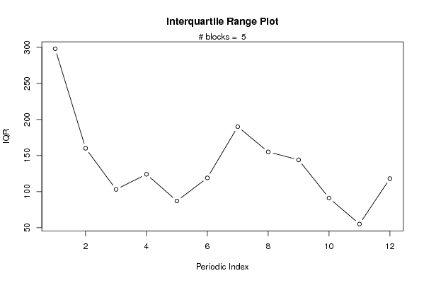
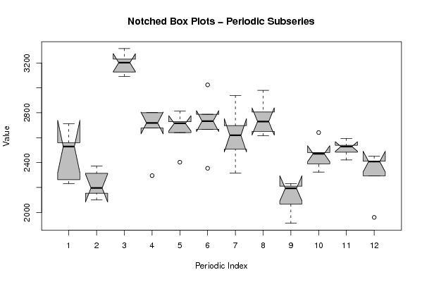
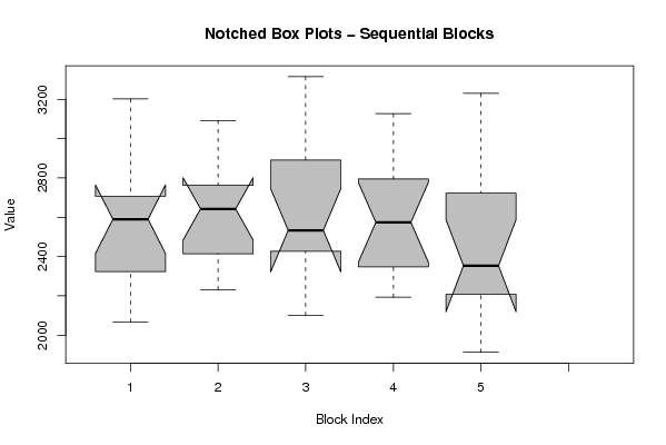
| Title produced by software | Standard Deviation Plot | ||||||||||||||||||||
| Date of computation | Tue, 29 Dec 2009 06:35:24 -0700 | ||||||||||||||||||||
| Cite this page as follows | Statistical Computations at FreeStatistics.org, Office for Research Development and Education, URL https://freestatistics.org/blog/index.php?v=date/2009/Dec/29/t12620938040yoqalmk7khai62.htm/, Retrieved Fri, 03 May 2024 13:35:50 +0000 | ||||||||||||||||||||
| Statistical Computations at FreeStatistics.org, Office for Research Development and Education, URL https://freestatistics.org/blog/index.php?pk=71117, Retrieved Fri, 03 May 2024 13:35:50 +0000 | |||||||||||||||||||||
| QR Codes: | |||||||||||||||||||||
|
| |||||||||||||||||||||
| Original text written by user: | |||||||||||||||||||||
| IsPrivate? | No (this computation is public) | ||||||||||||||||||||
| User-defined keywords | Paper | ||||||||||||||||||||
| Estimated Impact | 146 | ||||||||||||||||||||
Tree of Dependent Computations | |||||||||||||||||||||
| Family? (F = Feedback message, R = changed R code, M = changed R Module, P = changed Parameters, D = changed Data) | |||||||||||||||||||||
| - [Standard Deviation Plot] [3/11/2009] [2009-11-02 22:09:58] [b98453cac15ba1066b407e146608df68] - PD [Standard Deviation Plot] [ws6 range plot] [2009-11-06 16:04:51] [8b1aef4e7013bd33fbc2a5833375c5f5] - R PD [Standard Deviation Plot] [Standard_Deviatio...] [2009-12-29 13:35:24] [5b5bced41faf164488f2c271c918b21f] [Current] | |||||||||||||||||||||
| Feedback Forum | |||||||||||||||||||||
Post a new message | |||||||||||||||||||||
Dataset | |||||||||||||||||||||
| Dataseries X: | |||||||||||||||||||||
2529 2196 3202 2718 2728 2354 2697 2651 2067 2641 2539 2294 2712 2314 3092 2677 2813 2668 2939 2617 2231 2481 2421 2408 2560 2100 3315 2801 2403 3024 2507 2980 2211 2471 2594 2452 2232 2373 3127 2802 2641 2787 2619 2806 2193 2323 2529 2412 2262 2154 3230 2295 2715 2733 2317 2730 1913 2390 2484 1960 | |||||||||||||||||||||
Tables (Output of Computation) | |||||||||||||||||||||
| |||||||||||||||||||||
Figures (Output of Computation) | |||||||||||||||||||||
Input Parameters & R Code | |||||||||||||||||||||
| Parameters (Session): | |||||||||||||||||||||
| Parameters (R input): | |||||||||||||||||||||
| par1 = 12 ; | |||||||||||||||||||||
| R code (references can be found in the software module): | |||||||||||||||||||||
par1 <- as.numeric(par1) | |||||||||||||||||||||