Free Statistics
of Irreproducible Research!
Description of Statistical Computation | |||||||||||||||||||||||||||||||||||||||||||||||||||||
|---|---|---|---|---|---|---|---|---|---|---|---|---|---|---|---|---|---|---|---|---|---|---|---|---|---|---|---|---|---|---|---|---|---|---|---|---|---|---|---|---|---|---|---|---|---|---|---|---|---|---|---|---|---|
| Author's title | |||||||||||||||||||||||||||||||||||||||||||||||||||||
| Author | *The author of this computation has been verified* | ||||||||||||||||||||||||||||||||||||||||||||||||||||
| R Software Module | rwasp_edauni.wasp | ||||||||||||||||||||||||||||||||||||||||||||||||||||
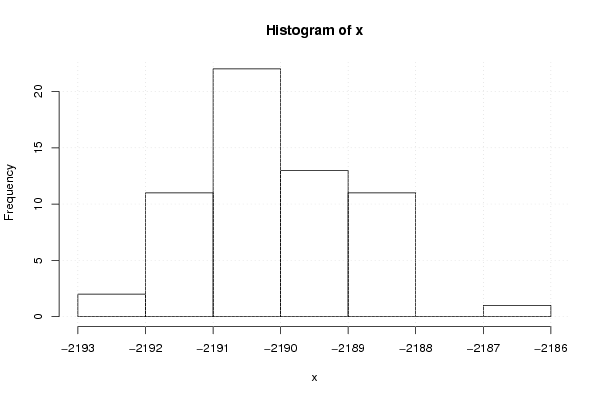
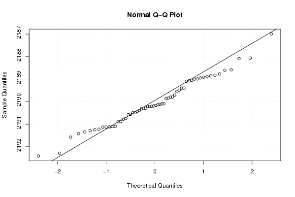
| Title produced by software | Univariate Explorative Data Analysis | ||||||||||||||||||||||||||||||||||||||||||||||||||||
| Date of computation | Mon, 28 Dec 2009 06:10:54 -0700 | ||||||||||||||||||||||||||||||||||||||||||||||||||||
| Cite this page as follows | Statistical Computations at FreeStatistics.org, Office for Research Development and Education, URL https://freestatistics.org/blog/index.php?v=date/2009/Dec/28/t12620059177ut4jaojtf1bekk.htm/, Retrieved Sun, 05 May 2024 12:44:21 +0000 | ||||||||||||||||||||||||||||||||||||||||||||||||||||
| Statistical Computations at FreeStatistics.org, Office for Research Development and Education, URL https://freestatistics.org/blog/index.php?pk=70953, Retrieved Sun, 05 May 2024 12:44:21 +0000 | |||||||||||||||||||||||||||||||||||||||||||||||||||||
| QR Codes: | |||||||||||||||||||||||||||||||||||||||||||||||||||||
|
| |||||||||||||||||||||||||||||||||||||||||||||||||||||
| Original text written by user: | |||||||||||||||||||||||||||||||||||||||||||||||||||||
| IsPrivate? | No (this computation is public) | ||||||||||||||||||||||||||||||||||||||||||||||||||||
| User-defined keywords | Paper | ||||||||||||||||||||||||||||||||||||||||||||||||||||
| Estimated Impact | 145 | ||||||||||||||||||||||||||||||||||||||||||||||||||||
Tree of Dependent Computations | |||||||||||||||||||||||||||||||||||||||||||||||||||||
| Family? (F = Feedback message, R = changed R code, M = changed R Module, P = changed Parameters, D = changed Data) | |||||||||||||||||||||||||||||||||||||||||||||||||||||
| - [Central Tendency] [SHW_WS3_Yt=c+Xt] [2009-10-16 08:10:06] [8b1aef4e7013bd33fbc2a5833375c5f5] - RMPD [Univariate Explorative Data Analysis] [] [2009-11-02 10:43:25] [8b1aef4e7013bd33fbc2a5833375c5f5] - R D [Univariate Explorative Data Analysis] [Run_sequence_et] [2009-12-28 13:10:54] [5b5bced41faf164488f2c271c918b21f] [Current] - RMPD [Harrell-Davis Quantiles] [Harrel-Davis_et] [2009-12-28 13:18:38] [2663058f2a5dda519058ac6b2228468f] - PD [Harrell-Davis Quantiles] [Harrel-Davis_et] [2009-12-28 13:49:16] [2663058f2a5dda519058ac6b2228468f] - PD [Harrell-Davis Quantiles] [Harrell-Davis_et] [2009-12-29 09:57:52] [2663058f2a5dda519058ac6b2228468f] | |||||||||||||||||||||||||||||||||||||||||||||||||||||
| Feedback Forum | |||||||||||||||||||||||||||||||||||||||||||||||||||||
Post a new message | |||||||||||||||||||||||||||||||||||||||||||||||||||||
Dataset | |||||||||||||||||||||||||||||||||||||||||||||||||||||
| Dataseries X: | |||||||||||||||||||||||||||||||||||||||||||||||||||||
-2188,94586 -2190,09434 -2186,99375 -2188,585139 -2188,606154 -2189,801223 -2188,827273 -2188,990937 -2190,774096 -2189,092814 -2189,398204 -2190,131737 -2189 -2190,292754 -2188,063584 -2189,394886 -2189,076056 -2189,547486 -2188,858726 -2189,790634 -2190,870879 -2190,20274 -2190,385246 -2190,491892 -2190,09973 -2191,339623 -2188,08871 -2189,490617 -2190,557641 -2188,914439 -2190,314667 -2189,053333 -2191,119681 -2190,428191 -2190,119363 -2190,496021 -2191,095238 -2190,738786 -2188,771053 -2189,703125 -2190,210797 -2189,853846 -2190,30179 -2189,841837 -2191,419847 -2191,104061 -2190,581218 -2190,893671 -2191,287879 -2191,574307 -2188,884422 -2191,24812 -2190,2125 -2190,1675 -2191,221945 -2190,19202 -2192,288177 -2191,127764 -2191,12766 -2192,409836 | |||||||||||||||||||||||||||||||||||||||||||||||||||||
Tables (Output of Computation) | |||||||||||||||||||||||||||||||||||||||||||||||||||||
| |||||||||||||||||||||||||||||||||||||||||||||||||||||
Figures (Output of Computation) | |||||||||||||||||||||||||||||||||||||||||||||||||||||
Input Parameters & R Code | |||||||||||||||||||||||||||||||||||||||||||||||||||||
| Parameters (Session): | |||||||||||||||||||||||||||||||||||||||||||||||||||||
| par1 = 0 ; par2 = 36 ; | |||||||||||||||||||||||||||||||||||||||||||||||||||||
| Parameters (R input): | |||||||||||||||||||||||||||||||||||||||||||||||||||||
| par1 = 0 ; par2 = 36 ; | |||||||||||||||||||||||||||||||||||||||||||||||||||||
| R code (references can be found in the software module): | |||||||||||||||||||||||||||||||||||||||||||||||||||||
par1 <- as.numeric(par1) | |||||||||||||||||||||||||||||||||||||||||||||||||||||