Free Statistics
of Irreproducible Research!
Description of Statistical Computation | |||||||||||||||||||||
|---|---|---|---|---|---|---|---|---|---|---|---|---|---|---|---|---|---|---|---|---|---|
| Author's title | |||||||||||||||||||||
| Author | *The author of this computation has been verified* | ||||||||||||||||||||
| R Software Module | rwasp_sdplot.wasp | ||||||||||||||||||||
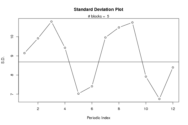
| Title produced by software | Standard Deviation Plot | ||||||||||||||||||||
| Date of computation | Wed, 23 Dec 2009 09:24:59 -0700 | ||||||||||||||||||||
| Cite this page as follows | Statistical Computations at FreeStatistics.org, Office for Research Development and Education, URL https://freestatistics.org/blog/index.php?v=date/2009/Dec/23/t1261585540c6y5cq37nsa9thi.htm/, Retrieved Mon, 29 Apr 2024 08:47:40 +0000 | ||||||||||||||||||||
| Statistical Computations at FreeStatistics.org, Office for Research Development and Education, URL https://freestatistics.org/blog/index.php?pk=70552, Retrieved Mon, 29 Apr 2024 08:47:40 +0000 | |||||||||||||||||||||
| QR Codes: | |||||||||||||||||||||
|
| |||||||||||||||||||||
| Original text written by user: | |||||||||||||||||||||
| IsPrivate? | No (this computation is public) | ||||||||||||||||||||
| User-defined keywords | |||||||||||||||||||||
| Estimated Impact | 94 | ||||||||||||||||||||
Tree of Dependent Computations | |||||||||||||||||||||
| Family? (F = Feedback message, R = changed R code, M = changed R Module, P = changed Parameters, D = changed Data) | |||||||||||||||||||||
| - [Standard Deviation Plot] [3/11/2009] [2009-11-02 22:09:58] [b98453cac15ba1066b407e146608df68] - PD [Standard Deviation Plot] [Workshop 6: Stand...] [2009-12-23 16:24:59] [d41d8cd98f00b204e9800998ecf8427e] [Current] | |||||||||||||||||||||
| Feedback Forum | |||||||||||||||||||||
Post a new message | |||||||||||||||||||||
Dataset | |||||||||||||||||||||
| Dataseries X: | |||||||||||||||||||||
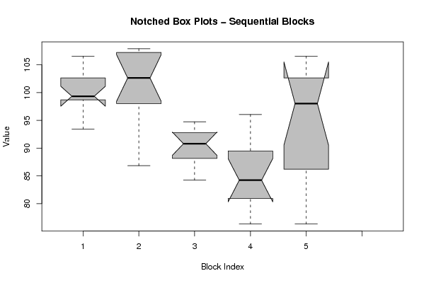
106.5789 101.3158 98.68421 100 102.6316 102.6316 102.6316 98.68421 98.68421 93.42105 98.68421 98.68421 100 101.3158 101.3158 103.9474 106.5789 107.8947 107.8947 107.8947 103.9474 96.05263 90.78947 86.84211 88.15789 90.78947 92.10526 93.42105 94.73684 93.42105 90.78947 92.10526 89.47368 84.21053 88.15789 86.84211 84.21053 82.89474 81.57895 85.52632 89.47368 89.47368 84.21053 80.26316 76.31579 80.26316 94.73684 96.05263 90.78947 80.26316 76.31579 81.57895 93.42105 101.3158 103.9474 101.3158 97.36842 98.68421 105.2632 106.5789 | |||||||||||||||||||||
Tables (Output of Computation) | |||||||||||||||||||||
| |||||||||||||||||||||
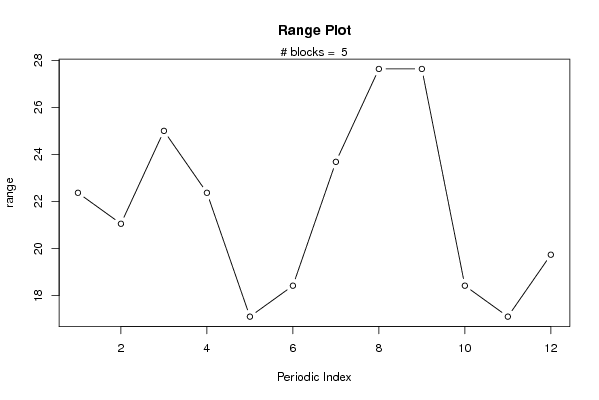
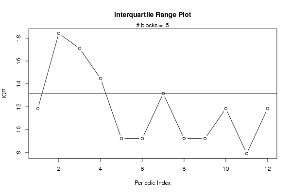
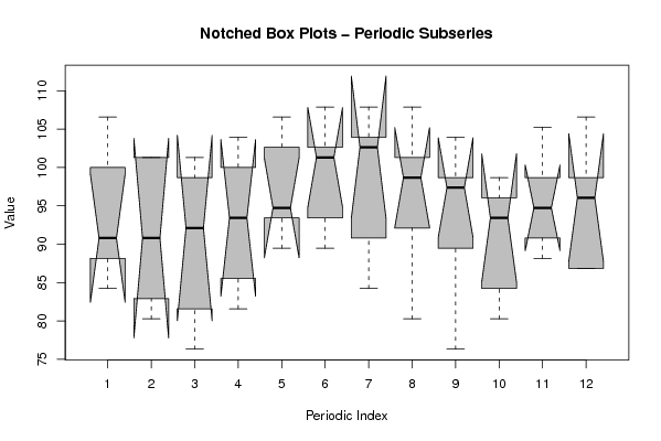
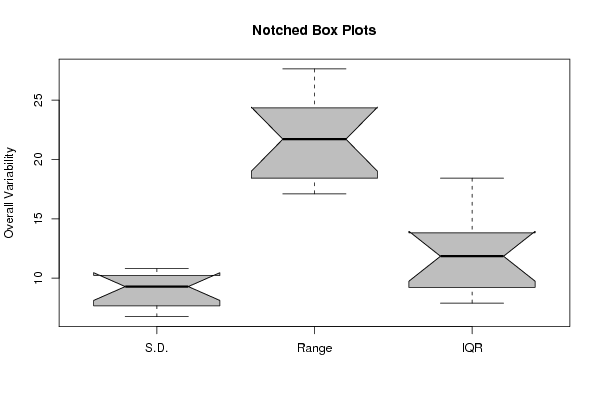
Figures (Output of Computation) | |||||||||||||||||||||
Input Parameters & R Code | |||||||||||||||||||||
| Parameters (Session): | |||||||||||||||||||||
| par1 = 12 ; | |||||||||||||||||||||
| Parameters (R input): | |||||||||||||||||||||
| par1 = 12 ; | |||||||||||||||||||||
| R code (references can be found in the software module): | |||||||||||||||||||||
par1 <- as.numeric(par1) | |||||||||||||||||||||