Free Statistics
of Irreproducible Research!
Description of Statistical Computation | |||||||||||||||||||||||||||||||||||||||||||||
|---|---|---|---|---|---|---|---|---|---|---|---|---|---|---|---|---|---|---|---|---|---|---|---|---|---|---|---|---|---|---|---|---|---|---|---|---|---|---|---|---|---|---|---|---|---|
| Author's title | |||||||||||||||||||||||||||||||||||||||||||||
| Author | *The author of this computation has been verified* | ||||||||||||||||||||||||||||||||||||||||||||
| R Software Module | rwasp_bidensity.wasp | ||||||||||||||||||||||||||||||||||||||||||||
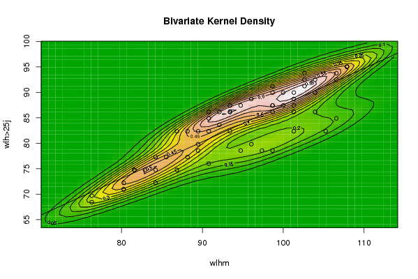
| Title produced by software | Bivariate Kernel Density Estimation | ||||||||||||||||||||||||||||||||||||||||||||
| Date of computation | Wed, 23 Dec 2009 08:59:17 -0700 | ||||||||||||||||||||||||||||||||||||||||||||
| Cite this page as follows | Statistical Computations at FreeStatistics.org, Office for Research Development and Education, URL https://freestatistics.org/blog/index.php?v=date/2009/Dec/23/t1261584043yrrmwebrh4yohtd.htm/, Retrieved Mon, 29 Apr 2024 15:03:28 +0000 | ||||||||||||||||||||||||||||||||||||||||||||
| Statistical Computations at FreeStatistics.org, Office for Research Development and Education, URL https://freestatistics.org/blog/index.php?pk=70547, Retrieved Mon, 29 Apr 2024 15:03:28 +0000 | |||||||||||||||||||||||||||||||||||||||||||||
| QR Codes: | |||||||||||||||||||||||||||||||||||||||||||||
|
| |||||||||||||||||||||||||||||||||||||||||||||
| Original text written by user: | |||||||||||||||||||||||||||||||||||||||||||||
| IsPrivate? | No (this computation is public) | ||||||||||||||||||||||||||||||||||||||||||||
| User-defined keywords | |||||||||||||||||||||||||||||||||||||||||||||
| Estimated Impact | 103 | ||||||||||||||||||||||||||||||||||||||||||||
Tree of Dependent Computations | |||||||||||||||||||||||||||||||||||||||||||||
| Family? (F = Feedback message, R = changed R code, M = changed R Module, P = changed Parameters, D = changed Data) | |||||||||||||||||||||||||||||||||||||||||||||
| - [Bivariate Kernel Density Estimation] [3/11/2009] [2009-11-02 21:54:51] [b98453cac15ba1066b407e146608df68] - PD [Bivariate Kernel Density Estimation] [Workshop 6: Bivar...] [2009-12-23 15:59:17] [d41d8cd98f00b204e9800998ecf8427e] [Current] | |||||||||||||||||||||||||||||||||||||||||||||
| Feedback Forum | |||||||||||||||||||||||||||||||||||||||||||||
Post a new message | |||||||||||||||||||||||||||||||||||||||||||||
Dataset | |||||||||||||||||||||||||||||||||||||||||||||
| Dataseries X: | |||||||||||||||||||||||||||||||||||||||||||||
106.5789 101.3158 98.68421 100 102.6316 102.6316 102.6316 98.68421 98.68421 93.42105 98.68421 98.68421 100 101.3158 101.3158 103.9474 106.5789 107.8947 107.8947 107.8947 103.9474 96.05263 90.78947 86.84211 88.15789 90.78947 92.10526 93.42105 94.73684 93.42105 90.78947 92.10526 89.47368 84.21053 88.15789 86.84211 84.21053 82.89474 81.57895 85.52632 89.47368 89.47368 84.21053 80.26316 76.31579 80.26316 94.73684 96.05263 90.78947 80.26316 76.31579 81.57895 93.42105 101.3158 103.9474 101.3158 97.36842 98.68421 105.2632 106.5789 | |||||||||||||||||||||||||||||||||||||||||||||
| Dataseries Y: | |||||||||||||||||||||||||||||||||||||||||||||
93.76979937 89.96832101 86.16684266 87.43400211 91.23548046 93.76979937 92.50263992 87.43400211 87.43400211 86.16684266 89.96832101 91.23548046 89.96832101 88.70116156 87.43400211 89.96832101 92.50263992 95.03695882 95.03695882 95.03695882 92.50263992 88.70116156 84.89968321 82.36536431 82.36536431 82.36536431 83.63252376 86.16684266 87.43400211 87.43400211 86.16684266 86.16684266 82.36536431 77.2967265 77.2967265 74.7624076 72.2280887 74.7624076 74.7624076 77.2967265 79.83104541 78.56388596 74.7624076 72.2280887 68.42661035 70.96092925 78.56388596 79.83104541 76.02956705 70.96092925 69.6937698 74.7624076 82.36536431 86.16684266 86.16684266 82.36536431 78.56388596 78.56388596 82.36536431 84.89968321 | |||||||||||||||||||||||||||||||||||||||||||||
Tables (Output of Computation) | |||||||||||||||||||||||||||||||||||||||||||||
| |||||||||||||||||||||||||||||||||||||||||||||
Figures (Output of Computation) | |||||||||||||||||||||||||||||||||||||||||||||
Input Parameters & R Code | |||||||||||||||||||||||||||||||||||||||||||||
| Parameters (Session): | |||||||||||||||||||||||||||||||||||||||||||||
| par1 = 50 ; par2 = 50 ; par3 = 0 ; par4 = 0 ; par5 = 0 ; par6 = Y ; par7 = Y ; | |||||||||||||||||||||||||||||||||||||||||||||
| Parameters (R input): | |||||||||||||||||||||||||||||||||||||||||||||
| par1 = 50 ; par2 = 50 ; par3 = 0 ; par4 = 0 ; par5 = 0 ; par6 = Y ; par7 = Y ; | |||||||||||||||||||||||||||||||||||||||||||||
| R code (references can be found in the software module): | |||||||||||||||||||||||||||||||||||||||||||||
par1 <- as(par1,'numeric') | |||||||||||||||||||||||||||||||||||||||||||||