Free Statistics
of Irreproducible Research!
Description of Statistical Computation | |||||||||||||||||||||||||||||||||||||||||||||||||||||||||||||||||
|---|---|---|---|---|---|---|---|---|---|---|---|---|---|---|---|---|---|---|---|---|---|---|---|---|---|---|---|---|---|---|---|---|---|---|---|---|---|---|---|---|---|---|---|---|---|---|---|---|---|---|---|---|---|---|---|---|---|---|---|---|---|---|---|---|---|
| Author's title | |||||||||||||||||||||||||||||||||||||||||||||||||||||||||||||||||
| Author | *The author of this computation has been verified* | ||||||||||||||||||||||||||||||||||||||||||||||||||||||||||||||||
| R Software Module | rwasp_edabi.wasp | ||||||||||||||||||||||||||||||||||||||||||||||||||||||||||||||||
| Title produced by software | Bivariate Explorative Data Analysis | ||||||||||||||||||||||||||||||||||||||||||||||||||||||||||||||||
| Date of computation | Sat, 19 Dec 2009 12:10:37 -0700 | ||||||||||||||||||||||||||||||||||||||||||||||||||||||||||||||||
| Cite this page as follows | Statistical Computations at FreeStatistics.org, Office for Research Development and Education, URL https://freestatistics.org/blog/index.php?v=date/2009/Dec/19/t12612500676i5crzrja3ghzi2.htm/, Retrieved Sun, 05 May 2024 16:31:29 +0000 | ||||||||||||||||||||||||||||||||||||||||||||||||||||||||||||||||
| Statistical Computations at FreeStatistics.org, Office for Research Development and Education, URL https://freestatistics.org/blog/index.php?pk=69734, Retrieved Sun, 05 May 2024 16:31:29 +0000 | |||||||||||||||||||||||||||||||||||||||||||||||||||||||||||||||||
| QR Codes: | |||||||||||||||||||||||||||||||||||||||||||||||||||||||||||||||||
|
| |||||||||||||||||||||||||||||||||||||||||||||||||||||||||||||||||
| Original text written by user: | |||||||||||||||||||||||||||||||||||||||||||||||||||||||||||||||||
| IsPrivate? | No (this computation is public) | ||||||||||||||||||||||||||||||||||||||||||||||||||||||||||||||||
| User-defined keywords | ShwPaper; bivariate EDA analyse | ||||||||||||||||||||||||||||||||||||||||||||||||||||||||||||||||
| Estimated Impact | 171 | ||||||||||||||||||||||||||||||||||||||||||||||||||||||||||||||||
Tree of Dependent Computations | |||||||||||||||||||||||||||||||||||||||||||||||||||||||||||||||||
| Family? (F = Feedback message, R = changed R code, M = changed R Module, P = changed Parameters, D = changed Data) | |||||||||||||||||||||||||||||||||||||||||||||||||||||||||||||||||
| - [Bivariate Data Series] [Bivariate dataset] [2008-01-05 23:51:08] [74be16979710d4c4e7c6647856088456] - RMPD [Bivariate Explorative Data Analysis] [Ws4 part 1.1 s090...] [2009-10-27 21:56:53] [e0fc65a5811681d807296d590d5b45de] - M D [Bivariate Explorative Data Analysis] [Paper; bivariate ...] [2009-12-19 19:10:37] [51108381f3361ca8af49c4f74052c840] [Current] - D [Bivariate Explorative Data Analysis] [PAPER EDA analyse] [2010-11-24 17:56:00] [814f53995537cd15c528d8efbf1cf544] - R PD [Bivariate Explorative Data Analysis] [PAPER DMA Bivaria...] [2010-12-08 16:59:16] [74be16979710d4c4e7c6647856088456] - RMPD [] [PAPER DMA Bivaria...] [-0001-11-30 00:00:00] [74be16979710d4c4e7c6647856088456] - RMPD [Univariate Data Series] [Data Xt paper dma] [2010-12-09 15:27:56] [2099aacba481f75a7f949aa310cab952] - RMPD [Univariate Data Series] [Data Yt paper DMA] [2010-12-09 15:34:47] [2099aacba481f75a7f949aa310cab952] - RMPD [Univariate Data Series] [Yt Gemiddelde aan...] [2010-12-09 15:43:19] [2099aacba481f75a7f949aa310cab952] - RMPD [Univariate Data Series] [Xt Gemiddelde oli...] [2010-12-09 15:45:25] [2099aacba481f75a7f949aa310cab952] - RMPD [Bivariate Explorative Data Analysis] [Biveriate EDA Pap...] [2010-12-09 15:48:00] [2099aacba481f75a7f949aa310cab952] - D [Bivariate Explorative Data Analysis] [] [2010-12-13 09:53:42] [1251ac2db27b84d4a3ba43449388906b] - [Bivariate Explorative Data Analysis] [workshop 10: Mult...] [2010-12-14 08:27:59] [814f53995537cd15c528d8efbf1cf544] - RMPD [Multiple Regression] [Multiple Regressi...] [2010-12-09 15:50:37] [2099aacba481f75a7f949aa310cab952] - RMPD [] [PAPER DMA Multipl...] [-0001-11-30 00:00:00] [74be16979710d4c4e7c6647856088456] - RMPD [] [PAPER DMA Multipl...] [-0001-11-30 00:00:00] [74be16979710d4c4e7c6647856088456] - RMPD [Cross Correlation Function] [cross correlation...] [2010-12-08 19:50:23] [74be16979710d4c4e7c6647856088456] - PD [Cross Correlation Function] [] [2010-12-09 09:22:26] [b98453cac15ba1066b407e146608df68] - D [Cross Correlation Function] [workshop 10] [2010-12-12 14:17:25] [717f3d787904f94c39256c5c1fc72d4c] - PD [Cross Correlation Function] [workshop 10] [2010-12-12 14:24:39] [717f3d787904f94c39256c5c1fc72d4c] - R PD [Cross Correlation Function] [CCF 3] [2010-12-14 17:53:52] [04d4386fa51dbd2ef12d0f1f80644886] - D [Cross Correlation Function] [] [2010-12-19 19:14:52] [de55ccbf69577500a5f46ed42a101114] - PD [Cross Correlation Function] [] [2010-12-09 09:25:48] [b98453cac15ba1066b407e146608df68] - R P [Cross Correlation Function] [PAPER DMA Cross C...] [2010-12-09 19:56:08] [2099aacba481f75a7f949aa310cab952] - P [Cross Correlation Function] [Paper DMA Cross C...] [2010-12-15 17:50:43] [2099aacba481f75a7f949aa310cab952] - RMPD [Variance Reduction Matrix] [PAPER DMA Varianc...] [2010-12-09 20:08:14] [2099aacba481f75a7f949aa310cab952] - RMPD [Variance Reduction Matrix] [PAPER DMA VRM Olie] [2010-12-09 20:10:17] [2099aacba481f75a7f949aa310cab952] - PD [Cross Correlation Function] [Cross validation ...] [2010-12-10 08:46:08] [aeb27d5c05332f2e597ad139ee63fbe4] - RMPD [Kendall tau Correlation Matrix] [WS10 Feedback Pea...] [2010-12-22 16:18:54] [abf4ff90b26c6b37be4a30063b404639] - RMPD [Kendall tau Correlation Matrix] [WS10 Feedback Ken...] [2010-12-22 16:20:27] [abf4ff90b26c6b37be4a30063b404639] - RMPD [Recursive Partitioning (Regression Trees)] [WS10 Feedback Rec...] [2010-12-22 16:40:24] [abf4ff90b26c6b37be4a30063b404639] - R D [Cross Correlation Function] [Paper/ Cross Corr...] [2010-12-10 14:13:23] [d59201e34006b7e3f71c33fa566f42b3] - R D [Cross Correlation Function] [CCF ] [2010-12-11 10:57:31] [04d4386fa51dbd2ef12d0f1f80644886] - D [Cross Correlation Function] [Cross Correlation...] [2010-12-11 15:22:29] [62f7c80c4d96454bbd2b2b026ea9aad9] - R D [Cross Correlation Function] [workshop 10] [2010-12-12 13:50:13] [717f3d787904f94c39256c5c1fc72d4c] - R PD [Cross Correlation Function] [CCF ] [2010-12-14 17:49:20] [04d4386fa51dbd2ef12d0f1f80644886] - RMPD [(Partial) Autocorrelation Function] [ACF aanvoerwaarde] [2010-12-16 11:01:16] [04d4386fa51dbd2ef12d0f1f80644886] - PD [Cross Correlation Function] [CCF aanvoer en aa...] [2010-12-16 10:58:21] [04d4386fa51dbd2ef12d0f1f80644886] - D [Cross Correlation Function] [] [2010-12-19 19:09:45] [de55ccbf69577500a5f46ed42a101114] - RMPD [Bivariate Granger Causality] [] [2010-12-09 09:27:32] [b98453cac15ba1066b407e146608df68] - PD [Bivariate Granger Causality] [Bivariate Granger...] [2010-12-10 08:56:43] [aeb27d5c05332f2e597ad139ee63fbe4] - PD [Bivariate Granger Causality] [workshop 10] [2010-12-12 14:35:01] [717f3d787904f94c39256c5c1fc72d4c] - PD [Bivariate Granger Causality] [workshop 10] [2010-12-12 14:36:35] [717f3d787904f94c39256c5c1fc72d4c] - R PD [Bivariate Granger Causality] [granger] [2010-12-14 17:56:45] [04d4386fa51dbd2ef12d0f1f80644886] - D [Bivariate Granger Causality] [] [2010-12-19 19:16:58] [de55ccbf69577500a5f46ed42a101114] - RMPD [Multiple Regression] [] [2010-12-09 09:37:57] [b98453cac15ba1066b407e146608df68] - D [Multiple Regression] [Multiple Regressi...] [2010-12-10 09:09:44] [aeb27d5c05332f2e597ad139ee63fbe4] - D [Multiple Regression] [workshop 10] [2010-12-12 20:47:37] [717f3d787904f94c39256c5c1fc72d4c] - R P [Multiple Regression] [Peer verbetering] [2010-12-17 17:37:09] [d6a5e6c1b0014d57cedb2bdfb4a7099f] - D [Multiple Regression] [] [2010-12-22 19:51:26] [de55ccbf69577500a5f46ed42a101114] - PD [Cross Correlation Function] [] [2010-12-09 09:43:43] [c2a9e95daa10045f9fd6252038bcb219] [Truncated] | |||||||||||||||||||||||||||||||||||||||||||||||||||||||||||||||||
| Feedback Forum | |||||||||||||||||||||||||||||||||||||||||||||||||||||||||||||||||
Post a new message | |||||||||||||||||||||||||||||||||||||||||||||||||||||||||||||||||
Dataset | |||||||||||||||||||||||||||||||||||||||||||||||||||||||||||||||||
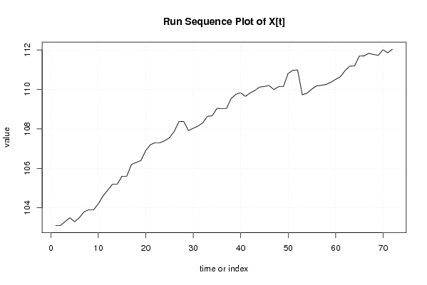
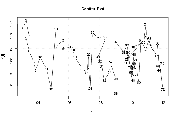
| Dataseries X: | |||||||||||||||||||||||||||||||||||||||||||||||||||||||||||||||||
103,1 103,1 103,3 103,5 103,3 103,5 103,8 103,9 103,9 104,2 104,6 104,9 105,2 105,2 105,6 105,6 106,2 106,3 106,4 106,9 107,2 107,3 107,3 107,4 107,55 107,87 108,37 108,38 107,92 108,03 108,14 108,3 108,64 108,66 109,04 109,03 109,03 109,54 109,75 109,83 109,65 109,82 109,95 110,12 110,15 110,2 109,99 110,14 110,14 110,81 110,97 110,99 109,73 109,81 110,02 110,18 110,21 110,25 110,36 110,51 110,64 110,95 111,18 111,19 111,69 111,7 111,83 111,77 111,73 112,01 111,86 112,04 | |||||||||||||||||||||||||||||||||||||||||||||||||||||||||||||||||
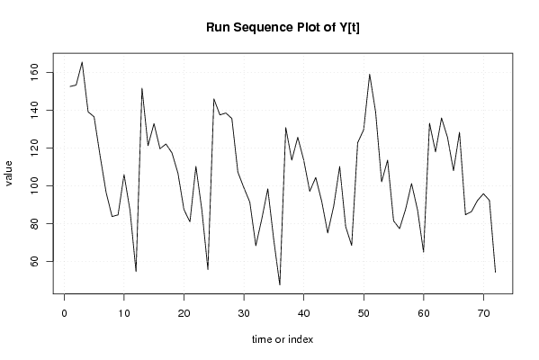
| Dataseries Y: | |||||||||||||||||||||||||||||||||||||||||||||||||||||||||||||||||
152,60 153,32 165,50 139,18 136,53 115,92 96,65 83,77 84,66 106,03 86,92 54,66 151,66 121,27 132,95 119,64 122,16 117,44 106,69 87,45 80,98 110,30 87,01 55,73 146,00 137,54 138,54 135,62 107,27 99,04 91,36 68,35 82,59 98,41 71,25 47,58 130,83 113,60 125,69 113,60 97,12 104,43 91,84 75,11 89,24 110,23 78,42 68,45 122,81 129,66 159,06 139,03 102,16 113,59 81,46 77,36 87,57 101,23 87,21 64,94 133,12 117,99 135,90 125,67 108,03 128,31 84,74 86,38 92,24 95,83 92,33 54,27 | |||||||||||||||||||||||||||||||||||||||||||||||||||||||||||||||||
Tables (Output of Computation) | |||||||||||||||||||||||||||||||||||||||||||||||||||||||||||||||||
| |||||||||||||||||||||||||||||||||||||||||||||||||||||||||||||||||
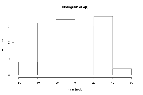
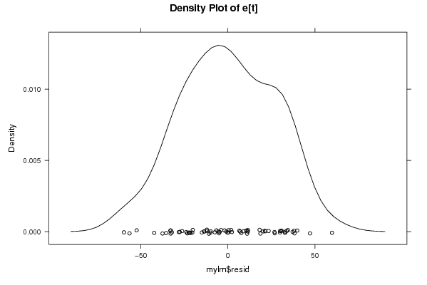
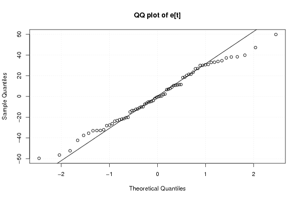
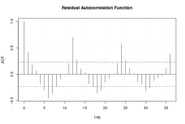
Figures (Output of Computation) | |||||||||||||||||||||||||||||||||||||||||||||||||||||||||||||||||
Input Parameters & R Code | |||||||||||||||||||||||||||||||||||||||||||||||||||||||||||||||||
| Parameters (Session): | |||||||||||||||||||||||||||||||||||||||||||||||||||||||||||||||||
| par1 = 0 ; par2 = 36 ; | |||||||||||||||||||||||||||||||||||||||||||||||||||||||||||||||||
| Parameters (R input): | |||||||||||||||||||||||||||||||||||||||||||||||||||||||||||||||||
| par1 = 0 ; par2 = 36 ; | |||||||||||||||||||||||||||||||||||||||||||||||||||||||||||||||||
| R code (references can be found in the software module): | |||||||||||||||||||||||||||||||||||||||||||||||||||||||||||||||||
par1 <- as.numeric(par1) | |||||||||||||||||||||||||||||||||||||||||||||||||||||||||||||||||