Free Statistics
of Irreproducible Research!
Description of Statistical Computation | |||||||||||||||||||||||||||||||||||||||||||||||||||||||||||||||||
|---|---|---|---|---|---|---|---|---|---|---|---|---|---|---|---|---|---|---|---|---|---|---|---|---|---|---|---|---|---|---|---|---|---|---|---|---|---|---|---|---|---|---|---|---|---|---|---|---|---|---|---|---|---|---|---|---|---|---|---|---|---|---|---|---|---|
| Author's title | |||||||||||||||||||||||||||||||||||||||||||||||||||||||||||||||||
| Author | *The author of this computation has been verified* | ||||||||||||||||||||||||||||||||||||||||||||||||||||||||||||||||
| R Software Module | rwasp_edabi.wasp | ||||||||||||||||||||||||||||||||||||||||||||||||||||||||||||||||
| Title produced by software | Bivariate Explorative Data Analysis | ||||||||||||||||||||||||||||||||||||||||||||||||||||||||||||||||
| Date of computation | Fri, 18 Dec 2009 07:51:48 -0700 | ||||||||||||||||||||||||||||||||||||||||||||||||||||||||||||||||
| Cite this page as follows | Statistical Computations at FreeStatistics.org, Office for Research Development and Education, URL https://freestatistics.org/blog/index.php?v=date/2009/Dec/18/t1261147985okwgkqcm0td6ni1.htm/, Retrieved Sat, 27 Apr 2024 20:25:43 +0000 | ||||||||||||||||||||||||||||||||||||||||||||||||||||||||||||||||
| Statistical Computations at FreeStatistics.org, Office for Research Development and Education, URL https://freestatistics.org/blog/index.php?pk=69385, Retrieved Sat, 27 Apr 2024 20:25:43 +0000 | |||||||||||||||||||||||||||||||||||||||||||||||||||||||||||||||||
| QR Codes: | |||||||||||||||||||||||||||||||||||||||||||||||||||||||||||||||||
|
| |||||||||||||||||||||||||||||||||||||||||||||||||||||||||||||||||
| Original text written by user: | |||||||||||||||||||||||||||||||||||||||||||||||||||||||||||||||||
| IsPrivate? | No (this computation is public) | ||||||||||||||||||||||||||||||||||||||||||||||||||||||||||||||||
| User-defined keywords | |||||||||||||||||||||||||||||||||||||||||||||||||||||||||||||||||
| Estimated Impact | 165 | ||||||||||||||||||||||||||||||||||||||||||||||||||||||||||||||||
Tree of Dependent Computations | |||||||||||||||||||||||||||||||||||||||||||||||||||||||||||||||||
| Family? (F = Feedback message, R = changed R code, M = changed R Module, P = changed Parameters, D = changed Data) | |||||||||||||||||||||||||||||||||||||||||||||||||||||||||||||||||
| - [Bivariate Data Series] [Bivariate dataset] [2008-01-05 23:51:08] [74be16979710d4c4e7c6647856088456] F RMPD [Univariate Explorative Data Analysis] [Colombia Coffee] [2008-01-07 14:21:11] [74be16979710d4c4e7c6647856088456] F RMPD [Univariate Data Series] [] [2009-10-14 08:30:28] [74be16979710d4c4e7c6647856088456] - RMPD [Partial Correlation] [Partial Correlation] [2009-12-16 14:03:17] [4d62210f0915d3a20cbf115865da7cd4] - D [Partial Correlation] [Partial Correlation] [2009-12-16 14:13:22] [4d62210f0915d3a20cbf115865da7cd4] - RMPD [Bivariate Explorative Data Analysis] [Bivariate EDA] [2009-12-18 14:26:54] [4d62210f0915d3a20cbf115865da7cd4] - D [Bivariate Explorative Data Analysis] [Autocorrelatie na...] [2009-12-18 14:51:48] [91df150cd527c563f0151b3a845ecd72] [Current] | |||||||||||||||||||||||||||||||||||||||||||||||||||||||||||||||||
| Feedback Forum | |||||||||||||||||||||||||||||||||||||||||||||||||||||||||||||||||
Post a new message | |||||||||||||||||||||||||||||||||||||||||||||||||||||||||||||||||
Dataset | |||||||||||||||||||||||||||||||||||||||||||||||||||||||||||||||||
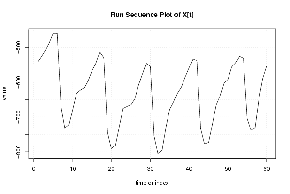
| Dataseries X: | |||||||||||||||||||||||||||||||||||||||||||||||||||||||||||||||||
-541,92 -525,95 -508,18 -487,35 -460,37 -460,77 -669,77 -731,59 -722,54 -678,58 -632,18 -622,86 -616,41 -595,08 -567,00 -546,17 -514,43 -530,00 -744,66 -790,91 -780,96 -726,99 -675,13 -669,87 -664,81 -648,05 -607,95 -577,31 -546,17 -554,39 -754,57 -804,78 -795,53 -731,15 -678,08 -657,36 -631,28 -614,61 -585,32 -559,84 -533,66 -537,62 -732,75 -776,80 -772,70 -720,64 -665,67 -639,99 -602,99 -591,98 -556,54 -544,37 -526,10 -531,06 -704,67 -738,21 -729,55 -648,80 -589,78 -554,99 | |||||||||||||||||||||||||||||||||||||||||||||||||||||||||||||||||
| Dataseries Y: | |||||||||||||||||||||||||||||||||||||||||||||||||||||||||||||||||
-540,33 -523,22 -503,80 -480,13 -452,36 -453,28 -661,26 -718,93 -712,26 -670,19 -623,90 -611,27 -602,79 -577,93 -552,90 -536,12 -504,48 -518,66 -732,24 -774,67 -772,03 -717,16 -662,92 -656,24 -649,06 -632,14 -592,99 -560,51 -525,84 -537,76 -733,93 -778,58 -772,77 -702,91 -652,63 -635,84 -607,10 -589,02 -556,86 -530,38 -506,83 -506,39 -695,70 -733,00 -732,26 -681,35 -631,57 -604,75 -562,64 -554,09 -522,00 -499,05 -481,10 -486,21 -654,56 -687,20 -689,68 -615,44 -557,36 -517,26 | |||||||||||||||||||||||||||||||||||||||||||||||||||||||||||||||||
Tables (Output of Computation) | |||||||||||||||||||||||||||||||||||||||||||||||||||||||||||||||||
| |||||||||||||||||||||||||||||||||||||||||||||||||||||||||||||||||
Figures (Output of Computation) | |||||||||||||||||||||||||||||||||||||||||||||||||||||||||||||||||
Input Parameters & R Code | |||||||||||||||||||||||||||||||||||||||||||||||||||||||||||||||||
| Parameters (Session): | |||||||||||||||||||||||||||||||||||||||||||||||||||||||||||||||||
| par1 = 0 ; par2 = 36 ; | |||||||||||||||||||||||||||||||||||||||||||||||||||||||||||||||||
| Parameters (R input): | |||||||||||||||||||||||||||||||||||||||||||||||||||||||||||||||||
| par1 = 0 ; par2 = 36 ; | |||||||||||||||||||||||||||||||||||||||||||||||||||||||||||||||||
| R code (references can be found in the software module): | |||||||||||||||||||||||||||||||||||||||||||||||||||||||||||||||||
par1 <- as.numeric(par1) | |||||||||||||||||||||||||||||||||||||||||||||||||||||||||||||||||