Free Statistics

of Irreproducible Research!

Author's title

Author*The author of this computation has been verified*
R Software Modulerwasp_edabi.wasp
Title produced by softwareBivariate Explorative Data Analysis
Date of computationFri, 18 Dec 2009 04:20:31 -0700
Cite this page as followsStatistical Computations at FreeStatistics.org, Office for Research Development and Education, URL https://freestatistics.org/blog/index.php?v=date/2009/Dec/18/t1261135275gar5nqg2ogur5sx.htm/, Retrieved Sat, 27 Apr 2024 23:59:06 +0000
Statistical Computations at FreeStatistics.org, Office for Research Development and Education, URL https://freestatistics.org/blog/index.php?pk=69240, Retrieved Sat, 27 Apr 2024 23:59:06 +0000
QR Codes:

Original text written by user:
IsPrivate?No (this computation is public)
User-defined keywords
Estimated Impact187
Family? (F = Feedback message, R = changed R code, M = changed R Module, P = changed Parameters, D = changed Data)
-       [Bivariate Explorative Data Analysis] [] [2009-12-18 11:20:31] [477c9cb8e7bda18f2375c22a66069c90] [Current]
Feedback Forum

Post a new message
Dataseries X:
8.1
7.7
7.5
7.6
7.8
7.8
7.8
7.5
7.5
7.1
7.5
7.5
7.6
7.7
7.7
7.9
8.1
8.2
8.2
8.2
7.9
7.3
6.9
6.6
6.7
6.9
7
7.1
7.2
7.1
6.9
7
6.8
6.4
6.7
6.6
6.4
6.3
6.2
6.5
6.8
6.8
6.4
6.1
5.8
6.1
7.2
7.3
6.9
6.1
5.8
6.2
7.1
7.7
7.9
7.7
7.4
7.5
8
8.1
8
Dataseries Y:
92.9
107.7
103.5
91.1
79.8
71.9
82.9
90.1
100.7
90.7
108.8
44.1
93.6
107.4
96.5
93.6
76.5
76.7
84
103.3
88.5
99
105.9
44.7
94
107.1
104.8
102.5
77.7
85.2
91.3
106.5
92.4
97.5
107
51.1
98.6
102.2
114.3
99.4
72.5
92.3
99.4
85.9
109.4
97.6
104.7
56.9
86.7
108.5
103.4
86.2
71
75.9
87.1
102
88.5
87.8
100.8
50.6
85.9


Summary of computational transaction
Raw Inputview raw input (R code)
Raw Outputview raw output of R engine
Computing time5 seconds
R Server'Gwilym Jenkins' @ 72.249.127.135

\begin{tabular}{lllllllll}
\hline
Summary of computational transaction \tabularnewline
Raw Input & view raw input (R code)  \tabularnewline
Raw Output & view raw output of R engine  \tabularnewline
Computing time & 5 seconds \tabularnewline
R Server & 'Gwilym Jenkins' @ 72.249.127.135 \tabularnewline
\hline
\end{tabular}
%Source: https://freestatistics.org/blog/index.php?pk=69240&T=0

[TABLE]
[ROW][C]Summary of computational transaction[/C][/ROW]
[ROW][C]Raw Input[/C][C]view raw input (R code) [/C][/ROW]
[ROW][C]Raw Output[/C][C]view raw output of R engine [/C][/ROW]
[ROW][C]Computing time[/C][C]5 seconds[/C][/ROW]
[ROW][C]R Server[/C][C]'Gwilym Jenkins' @ 72.249.127.135[/C][/ROW]
[/TABLE]
Source: https://freestatistics.org/blog/index.php?pk=69240&T=0

Globally Unique Identifier (entire table): ba.freestatistics.org/blog/index.php?pk=69240&T=0

As an alternative you can also use a QR Code:  

The GUIDs for individual cells are displayed in the table below:

Summary of computational transaction
Raw Inputview raw input (R code)
Raw Outputview raw output of R engine
Computing time5 seconds
R Server'Gwilym Jenkins' @ 72.249.127.135


Model: Y[t] = c + b X[t] + e[t]
c130.692426672635
b-5.59680206895694

\begin{tabular}{lllllllll}
\hline
Model: Y[t] = c + b X[t] + e[t] \tabularnewline
c & 130.692426672635 \tabularnewline
b & -5.59680206895694 \tabularnewline
\hline
\end{tabular}
%Source: https://freestatistics.org/blog/index.php?pk=69240&T=1

[TABLE]
[ROW][C]Model: Y[t] = c + b X[t] + e[t][/C][/ROW]
[ROW][C]c[/C][C]130.692426672635[/C][/ROW]
[ROW][C]b[/C][C]-5.59680206895694[/C][/ROW]
[/TABLE]
Source: https://freestatistics.org/blog/index.php?pk=69240&T=1

Globally Unique Identifier (entire table): ba.freestatistics.org/blog/index.php?pk=69240&T=1

As an alternative you can also use a QR Code:  

The GUIDs for individual cells are displayed in the table below:

Model: Y[t] = c + b X[t] + e[t]
c130.692426672635
b-5.59680206895694


Descriptive Statistics about e[t]
# observations61
minimum-49.053533017519
Q1-5.75513198304052
median2.02230967212504
mean-9.49673622645372e-17
Q311.9480659480025
maximum20.1029492583337

\begin{tabular}{lllllllll}
\hline
Descriptive Statistics about e[t] \tabularnewline
# observations & 61 \tabularnewline
minimum & -49.053533017519 \tabularnewline
Q1 & -5.75513198304052 \tabularnewline
median & 2.02230967212504 \tabularnewline
mean & -9.49673622645372e-17 \tabularnewline
Q3 & 11.9480659480025 \tabularnewline
maximum & 20.1029492583337 \tabularnewline
\hline
\end{tabular}
%Source: https://freestatistics.org/blog/index.php?pk=69240&T=2

[TABLE]
[ROW][C]Descriptive Statistics about e[t][/C][/ROW]
[ROW][C]# observations[/C][C]61[/C][/ROW]
[ROW][C]minimum[/C][C]-49.053533017519[/C][/ROW]
[ROW][C]Q1[/C][C]-5.75513198304052[/C][/ROW]
[ROW][C]median[/C][C]2.02230967212504[/C][/ROW]
[ROW][C]mean[/C][C]-9.49673622645372e-17[/C][/ROW]
[ROW][C]Q3[/C][C]11.9480659480025[/C][/ROW]
[ROW][C]maximum[/C][C]20.1029492583337[/C][/ROW]
[/TABLE]
Source: https://freestatistics.org/blog/index.php?pk=69240&T=2

Globally Unique Identifier (entire table): ba.freestatistics.org/blog/index.php?pk=69240&T=2

As an alternative you can also use a QR Code:  

The GUIDs for individual cells are displayed in the table below:

Descriptive Statistics about e[t]
# observations61
minimum-49.053533017519
Q1-5.75513198304052
median2.02230967212504
mean-9.49673622645372e-17
Q311.9480659480025
maximum20.1029492583337


Parameters (Session):
par1 = 0 ; par2 = 36 ;
Parameters (R input):
par1 = 0 ; par2 = 36 ;
R code (references can be found in the software module):
par1 <- as.numeric(par1)
par2 <- as.numeric(par2)
x <- as.ts(x)
y <- as.ts(y)
mylm <- lm(y~x)
cbind(mylm$resid)
library(lattice)
bitmap(file='pic1.png')
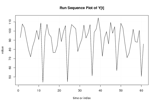
plot(y,type='l',main='Run Sequence Plot of Y[t]',xlab='time or index',ylab='value')
grid()
dev.off()
bitmap(file='pic1a.png')
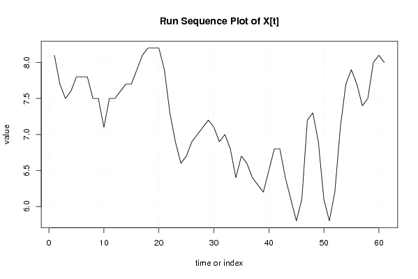
plot(x,type='l',main='Run Sequence Plot of X[t]',xlab='time or index',ylab='value')
grid()
dev.off()
bitmap(file='pic1b.png')
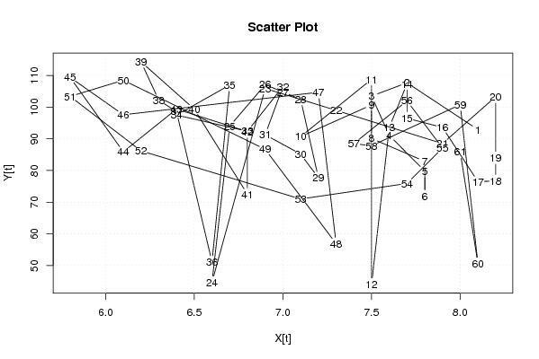
plot(x,y,main='Scatter Plot',xlab='X[t]',ylab='Y[t]')
grid()
dev.off()
bitmap(file='pic1c.png')
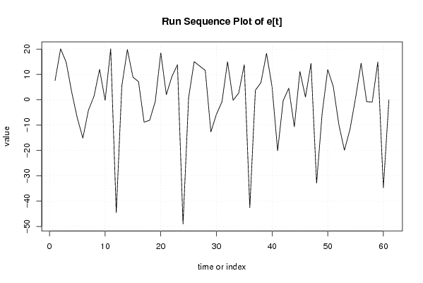
plot(mylm$resid,type='l',main='Run Sequence Plot of e[t]',xlab='time or index',ylab='value')
grid()
dev.off()
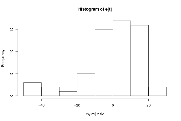
bitmap(file='pic2.png')
hist(mylm$resid,main='Histogram of e[t]')
dev.off()
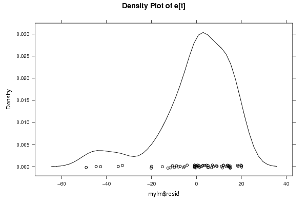
bitmap(file='pic3.png')
if (par1 > 0)
{
densityplot(~mylm$resid,col='black',main=paste('Density Plot of e[t] bw = ',par1),bw=par1)
} else {
densityplot(~mylm$resid,col='black',main='Density Plot of e[t]')
}
dev.off()
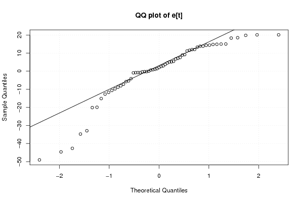
bitmap(file='pic4.png')
qqnorm(mylm$resid,main='QQ plot of e[t]')
qqline(mylm$resid)
grid()
dev.off()
if (par2 > 0)
{
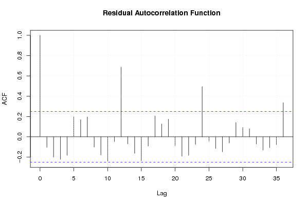
bitmap(file='pic5.png')
acf(mylm$resid,lag.max=par2,main='Residual Autocorrelation Function')
grid()
dev.off()
}
summary(x)
load(file='createtable')
a<-table.start()
a<-table.row.start(a)
a<-table.element(a,'Model: Y[t] = c + b X[t] + e[t]',2,TRUE)
a<-table.row.end(a)
a<-table.row.start(a)
a<-table.element(a,'c',1,TRUE)
a<-table.element(a,mylm$coeff[[1]])
a<-table.row.end(a)
a<-table.row.start(a)
a<-table.element(a,'b',1,TRUE)
a<-table.element(a,mylm$coeff[[2]])
a<-table.row.end(a)
a<-table.end(a)
table.save(a,file='mytable.tab')
a<-table.start()
a<-table.row.start(a)
a<-table.element(a,'Descriptive Statistics about e[t]',2,TRUE)
a<-table.row.end(a)
a<-table.row.start(a)
a<-table.element(a,'# observations',header=TRUE)
a<-table.element(a,length(mylm$resid))
a<-table.row.end(a)
a<-table.row.start(a)
a<-table.element(a,'minimum',header=TRUE)
a<-table.element(a,min(mylm$resid))
a<-table.row.end(a)
a<-table.row.start(a)
a<-table.element(a,'Q1',header=TRUE)
a<-table.element(a,quantile(mylm$resid,0.25))
a<-table.row.end(a)
a<-table.row.start(a)
a<-table.element(a,'median',header=TRUE)
a<-table.element(a,median(mylm$resid))
a<-table.row.end(a)
a<-table.row.start(a)
a<-table.element(a,'mean',header=TRUE)
a<-table.element(a,mean(mylm$resid))
a<-table.row.end(a)
a<-table.row.start(a)
a<-table.element(a,'Q3',header=TRUE)
a<-table.element(a,quantile(mylm$resid,0.75))
a<-table.row.end(a)
a<-table.row.start(a)
a<-table.element(a,'maximum',header=TRUE)
a<-table.element(a,max(mylm$resid))
a<-table.row.end(a)
a<-table.end(a)
table.save(a,file='mytable.tab')