Repository of Reproducible Computations

Free Statistics

of Irreproducible Research!

Author's title

Author

*The author of this computation has been verified*

R Software Module

rwasp_notchedbox1.wasp

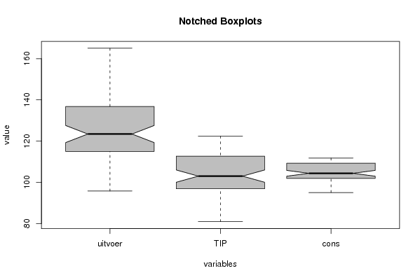
Title produced by software

Notched Boxplots

Date of computation

Fri, 18 Dec 2009 02:21:15 -0700

Cite this page as follows

Statistical Computations at FreeStatistics.org, Office for Research Development and Education, URL https://freestatistics.org/blog/index.php?v=date/2009/Dec/18/t1261128111ehx5021n9opmce3.htm/, Retrieved Sat, 27 Apr 2024 20:12:53 +0000

Statistical Computations at FreeStatistics.org, Office for Research Development and Education, URL https://freestatistics.org/blog/index.php?pk=69176, Retrieved Sat, 27 Apr 2024 20:12:53 +0000

QR Codes:

Paste this QR Code to cite your computation.

Original text written by user:

IsPrivate?

No (this computation is public)

User-defined keywords

Estimated Impact

159

Family? (F = Feedback message, R = changed R code, M = changed R Module, P = changed Parameters, D = changed Data)

-       [Notched Boxplots] [Notched Boxplots 1] [2009-12-18 09:21:15] [0f1f1142419956a95ff6f880845f2408] [Current]
- R  D    [Notched Boxplots] [notched boxplot 1 ] [2012-12-14 18:45:13] [da21a4ad0d643c5ab6ae91160bdaaba7] 
-  M        [Notched Boxplots] [] [2012-12-19 22:55:07] [74be16979710d4c4e7c6647856088456] 
- R  D      [Notched Boxplots] [] [2012-12-19 23:02:58] [8c6900b6affe5ced50ee5724b2e31c80] 
- R  D      [Notched Boxplots] [] [2012-12-20 01:06:10] [8c6900b6affe5ced50ee5724b2e31c80] 
- R  D      [Notched Boxplots] [] [2012-12-20 01:20:24] [8c6900b6affe5ced50ee5724b2e31c80] 
- RMPD      [Histogram] [] [2012-12-20 01:38:31] [8c6900b6affe5ced50ee5724b2e31c80] 

Feedback Forum

Post a new message

Dataseries X:

Download CSV

Histogram

Boxplots

103,34	98,60	96,33
102,60	96,90	96,33
100,69	95,10	95,05
105,67	97,00	96,84
123,61	112,70	96,92
113,08	102,90	97,44
106,46	97,40	97,78
123,38	111,40	97,69
109,87	87,40	96,67
95,74	96,80	98,29
123,06	114,10	98,20
123,39	110,30	98,71
120,28	103,90	98,54
115,33	101,60	98,20
110,40	94,60	100,80
114,49	95,90	101,33
132,03	104,70	101,88
123,16	102,80	101,85
118,82	98,10	102,04
128,32	113,90	102,22
112,24	80,90	102,63
104,53	95,70	102,65
132,57	113,20	102,54
122,52	105,90	102,37
131,80	108,80	102,68
124,55	102,30	102,76
120,96	99,00	102,82
122,60	100,70	103,31
145,52	115,50	103,23
118,57	100,70	103,60
134,25	109,90	103,95
136,70	114,60	103,93
121,37	85,40	104,25
111,63	100,50	104,38
134,42	114,80	104,36
137,65	116,50	104,32
137,86	112,90	104,58
119,77	102,00	104,68
130,69	106,00	104,92
128,28	105,30	105,46
147,45	118,80	105,23
128,42	106,10	105,58
136,90	109,30	105,34
143,95	117,20	105,28
135,64	92,50	105,70
122,48	104,20	105,67
136,83	112,50	105,71
153,04	122,40	106,19
142,71	113,30	106,93
123,46	100,00	107,44
144,37	110,70	107,85
146,15	112,80	108,71
147,61	109,80	109,32
158,51	117,30	109,49
147,40	109,10	110,20
165,05	115,90	110,62
154,64	96,00	111,22
126,20	99,80	110,88
157,36	116,80	111,15
154,15	115,70	111,29
123,21	99,40	111,09
113,07	94,30	111,24
110,45	91,00	111,45
113,57	93,20	111,75
122,44	103,10	111,07
114,93	94,10	111,17
111,85	91,80	110,96
126,04	102,70	110,50
121,34	82,60	110,48
124,36	89,10	110,66

Summary of computational transaction
Raw Input	view raw input (R code)
Raw Output	view raw output of R engine
Computing time	1 seconds
R Server	'Gwilym Jenkins' @ 72.249.127.135

\begin{tabular}{lllllllll}
\hline
Summary of computational transaction \tabularnewline
Raw Input & view raw input (R code)  \tabularnewline
Raw Output & view raw output of R engine  \tabularnewline
Computing time & 1 seconds \tabularnewline
R Server & 'Gwilym Jenkins' @ 72.249.127.135 \tabularnewline
\hline
\end{tabular}
%Source: https://freestatistics.org/blog/index.php?pk=69176&T=0

[TABLE]
[ROW][C]Summary of computational transaction[/C][/ROW]
[ROW][C]Raw Input[/C][C]view raw input (R code) [/C][/ROW]
[ROW][C]Raw Output[/C][C]view raw output of R engine [/C][/ROW]
[ROW][C]Computing time[/C][C]1 seconds[/C][/ROW]
[ROW][C]R Server[/C][C]'Gwilym Jenkins' @ 72.249.127.135[/C][/ROW]
[/TABLE]
Source: https://freestatistics.org/blog/index.php?pk=69176&T=0

Globally Unique Identifier (entire table): ba.freestatistics.org/blog/index.php?pk=69176&T=0

As an alternative you can also use a QR Code:

The GUIDs for individual cells are displayed in the table below:

Summary of computational transaction
Raw Input	view raw input (R code)
Raw Output	view raw output of R engine
Computing time	1 seconds
R Server	'Gwilym Jenkins' @ 72.249.127.135

Boxplot statistics
Variable	lower whisker	lower hinge	median	upper hinge	upper whisker
uitvoer	95.74	114.93	123.425	136.83	165.05
TIP	80.9	96.9	103	112.7	122.4
cons	95.05	101.88	104.37	109.32	111.75

\begin{tabular}{lllllllll}
\hline
Boxplot statistics \tabularnewline
Variable & lower whisker & lower hinge & median & upper hinge & upper whisker \tabularnewline
uitvoer & 95.74 & 114.93 & 123.425 & 136.83 & 165.05 \tabularnewline
TIP & 80.9 & 96.9 & 103 & 112.7 & 122.4 \tabularnewline
cons & 95.05 & 101.88 & 104.37 & 109.32 & 111.75 \tabularnewline
\hline
\end{tabular}
%Source: https://freestatistics.org/blog/index.php?pk=69176&T=1

[TABLE]
[ROW][C]Boxplot statistics[/C][/ROW]
[ROW][C]Variable[/C][C]lower whisker[/C][C]lower hinge[/C][C]median[/C][C]upper hinge[/C][C]upper whisker[/C][/ROW]
[ROW][C]uitvoer[/C][C]95.74[/C][C]114.93[/C][C]123.425[/C][C]136.83[/C][C]165.05[/C][/ROW]
[ROW][C]TIP[/C][C]80.9[/C][C]96.9[/C][C]103[/C][C]112.7[/C][C]122.4[/C][/ROW]
[ROW][C]cons[/C][C]95.05[/C][C]101.88[/C][C]104.37[/C][C]109.32[/C][C]111.75[/C][/ROW]
[/TABLE]
Source: https://freestatistics.org/blog/index.php?pk=69176&T=1

Globally Unique Identifier (entire table): ba.freestatistics.org/blog/index.php?pk=69176&T=1

As an alternative you can also use a QR Code:

The GUIDs for individual cells are displayed in the table below:

Boxplot statistics
Variable	lower whisker	lower hinge	median	upper hinge	upper whisker
uitvoer	95.74	114.93	123.425	136.83	165.05
TIP	80.9	96.9	103	112.7	122.4
cons	95.05	101.88	104.37	109.32	111.75

Boxplot Notches
Variable	lower bound	median	upper bound
uitvoer	119.289269965981	123.425	127.560730034019
TIP	100.016231299658	103	105.983768700342
cons	102.964984865155	104.37	105.775015134845

\begin{tabular}{lllllllll}
\hline
Boxplot Notches \tabularnewline
Variable & lower bound & median & upper bound \tabularnewline
uitvoer & 119.289269965981 & 123.425 & 127.560730034019 \tabularnewline
TIP & 100.016231299658 & 103 & 105.983768700342 \tabularnewline
cons & 102.964984865155 & 104.37 & 105.775015134845 \tabularnewline
\hline
\end{tabular}
%Source: https://freestatistics.org/blog/index.php?pk=69176&T=2

[TABLE]
[ROW][C]Boxplot Notches[/C][/ROW]
[ROW][C]Variable[/C][C]lower bound[/C][C]median[/C][C]upper bound[/C][/ROW]
[ROW][C]uitvoer[/C][C]119.289269965981[/C][C]123.425[/C][C]127.560730034019[/C][/ROW]
[ROW][C]TIP[/C][C]100.016231299658[/C][C]103[/C][C]105.983768700342[/C][/ROW]
[ROW][C]cons[/C][C]102.964984865155[/C][C]104.37[/C][C]105.775015134845[/C][/ROW]
[/TABLE]
Source: https://freestatistics.org/blog/index.php?pk=69176&T=2

Globally Unique Identifier (entire table): ba.freestatistics.org/blog/index.php?pk=69176&T=2

As an alternative you can also use a QR Code:

The GUIDs for individual cells are displayed in the table below:

Boxplot Notches
Variable	lower bound	median	upper bound
uitvoer	119.289269965981	123.425	127.560730034019
TIP	100.016231299658	103	105.983768700342
cons	102.964984865155	104.37	105.775015134845

Figure 1

PNG link

Postscript link

PDF link

Parameters (Session):

par1 = grey ;

Parameters (R input):

par1 = grey ;

R code (references can be found in the software module):

z <- as.data.frame(t(y))
bitmap(file='test1.png')
(r<-boxplot(z ,xlab=xlab,ylab=ylab,main=main,notch=TRUE,col=par1))
dev.off()
load(file='createtable')
a<-table.start()
a<-table.row.start(a)
a<-table.element(a,hyperlink('overview.htm','Boxplot statistics','Boxplot overview'),6,TRUE)
a<-table.row.end(a)
a<-table.row.start(a)
a<-table.element(a,'Variable',1,TRUE)
a<-table.element(a,hyperlink('lower_whisker.htm','lower whisker','definition of lower whisker'),1,TRUE)
a<-table.element(a,hyperlink('lower_hinge.htm','lower hinge','definition of lower hinge'),1,TRUE)
a<-table.element(a,hyperlink('central_tendency.htm','median','definitions about measures of central tendency'),1,TRUE)
a<-table.element(a,hyperlink('upper_hinge.htm','upper hinge','definition of upper hinge'),1,TRUE)
a<-table.element(a,hyperlink('upper_whisker.htm','upper whisker','definition of upper whisker'),1,TRUE)
a<-table.row.end(a)
for (i in 1:length(y[,1]))
{
a<-table.row.start(a)
a<-table.element(a,dimnames(t(x))[[2]][i],1,TRUE)
for (j in 1:5)
{
a<-table.element(a,r$stats[j,i])
}
a<-table.row.end(a)
}
a<-table.end(a)
table.save(a,file='mytable.tab')
a<-table.start()
a<-table.row.start(a)
a<-table.element(a,'Boxplot Notches',4,TRUE)
a<-table.row.end(a)
a<-table.row.start(a)
a<-table.element(a,'Variable',1,TRUE)
a<-table.element(a,'lower bound',1,TRUE)
a<-table.element(a,'median',1,TRUE)
a<-table.element(a,'upper bound',1,TRUE)
a<-table.row.end(a)
for (i in 1:length(y[,1]))
{
a<-table.row.start(a)
a<-table.element(a,dimnames(t(x))[[2]][i],1,TRUE)
a<-table.element(a,r$conf[1,i])
a<-table.element(a,r$stats[3,i])
a<-table.element(a,r$conf[2,i])
a<-table.row.end(a)
}
a<-table.end(a)
table.save(a,file='mytable1.tab')

Free Statistics

Description of Statistical Computation

Tree of Dependent Computations

Dataset

Tables (Output of Computation)

Figures (Output of Computation)

Input Parameters & R Code