Repository of Reproducible Computations

Free Statistics

of Irreproducible Research!

Author's title

Author

*The author of this computation has been verified*

R Software Module

rwasp_autocorrelation.wasp

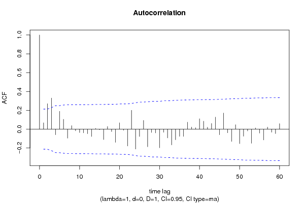
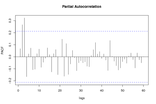
Title produced by software

(Partial) Autocorrelation Function

Date of computation

Wed, 16 Dec 2009 13:41:59 -0700

Cite this page as follows

Statistical Computations at FreeStatistics.org, Office for Research Development and Education, URL https://freestatistics.org/blog/index.php?v=date/2009/Dec/16/t12609961931k208s8qb582qlc.htm/, Retrieved Tue, 30 Apr 2024 16:10:07 +0000

Statistical Computations at FreeStatistics.org, Office for Research Development and Education, URL https://freestatistics.org/blog/index.php?pk=68595, Retrieved Tue, 30 Apr 2024 16:10:07 +0000

QR Codes:

Paste this QR Code to cite your computation.

Original text written by user:

IsPrivate?

No (this computation is public)

User-defined keywords

Estimated Impact

117

Family? (F = Feedback message, R = changed R code, M = changed R Module, P = changed Parameters, D = changed Data)

-     [Bivariate Explorative Data Analysis] [Paper Bivariate E...] [2009-12-13 14:39:24] [143cbdcaf7333bdd9926a1dde50d1082]
- RMPD  [(Partial) Autocorrelation Function] [Paper-ACF2-Yt] [2009-12-15 17:59:21] [f15cfb7053d35072d573abca87df96a0]
-   P     [(Partial) Autocorrelation Function] [Paper-ACF3-Yt] [2009-12-15 18:09:38] [f15cfb7053d35072d573abca87df96a0]
- R  D        [(Partial) Autocorrelation Function] [Paper-ACF2-Xt] [2009-12-16 20:41:59] [5ed0eef5d4509bbfdac0ae6d87f3b4bf] [Current]

Feedback Forum

Post a new message

Dataseries X:

Download CSV

Histogram

Boxplots

Summary of computational transaction
Raw Input	view raw input (R code)
Raw Output	view raw output of R engine
Computing time	1 seconds
R Server	'Gwilym Jenkins' @ 72.249.127.135

\begin{tabular}{lllllllll}
\hline
Summary of computational transaction \tabularnewline
Raw Input & view raw input (R code)  \tabularnewline
Raw Output & view raw output of R engine  \tabularnewline
Computing time & 1 seconds \tabularnewline
R Server & 'Gwilym Jenkins' @ 72.249.127.135 \tabularnewline
\hline
\end{tabular}
%Source: https://freestatistics.org/blog/index.php?pk=68595&T=0

[TABLE]
[ROW][C]Summary of computational transaction[/C][/ROW]
[ROW][C]Raw Input[/C][C]view raw input (R code) [/C][/ROW]
[ROW][C]Raw Output[/C][C]view raw output of R engine [/C][/ROW]
[ROW][C]Computing time[/C][C]1 seconds[/C][/ROW]
[ROW][C]R Server[/C][C]'Gwilym Jenkins' @ 72.249.127.135[/C][/ROW]
[/TABLE]
Source: https://freestatistics.org/blog/index.php?pk=68595&T=0

Globally Unique Identifier (entire table): ba.freestatistics.org/blog/index.php?pk=68595&T=0

As an alternative you can also use a QR Code:

The GUIDs for individual cells are displayed in the table below:

Summary of computational transaction
Raw Input	view raw input (R code)
Raw Output	view raw output of R engine
Computing time	1 seconds
R Server	'Gwilym Jenkins' @ 72.249.127.135

Autocorrelation Function
Time lag k	ACF(k)	T-STAT	P-value
1	0.067779	0.6249	0.266858
2	0.270187	2.491	0.007341
3	0.330274	3.045	0.001549
4	-0.059672	-0.5501	0.291831
5	0.189649	1.7485	0.041996
6	0.104661	0.9649	0.16866
7	-0.096391	-0.8887	0.18834
8	0.037217	0.3431	0.366178
9	-0.01795	-0.1655	0.434474
10	-0.036213	-0.3339	0.369653
11	-0.039796	-0.3669	0.357302
12	-0.049071	-0.4524	0.326061
13	-0.077849	-0.7177	0.237445
14	0.008221	0.0758	0.469882
15	-0.006461	-0.0596	0.47632
16	-0.110602	-1.0197	0.155381
17	0.028092	0.259	0.398132
18	-0.026244	-0.242	0.404697
19	-0.140439	-1.2948	0.099451
20	0.067355	0.621	0.268137
21	-0.012016	-0.1108	0.456027
22	-0.178771	-1.6482	0.051503
23	0.200073	1.8446	0.034291
24	-0.210995	-1.9453	0.027523
25	-0.07816	-0.7206	0.236567
26	0.093342	0.8606	0.195949
27	-0.186895	-1.7231	0.044255
28	-0.035394	-0.3263	0.372494
29	-0.039884	-0.3677	0.357002
30	-0.197527	-1.8211	0.036054
31	-0.03318	-0.3059	0.380212
32	-0.093388	-0.861	0.195832
33	-0.167224	-1.5417	0.063428
34	-0.113165	-1.0433	0.149877
35	-0.076606	-0.7063	0.240975
36	-0.07706	-0.7105	0.239684
37	0.073933	0.6816	0.248663
38	0.022441	0.2069	0.418295
39	0.015432	0.1423	0.4436
40	0.110587	1.0196	0.155416
41	0.084371	0.7779	0.219404
42	0.020569	0.1896	0.425024
43	0.060193	0.555	0.290191
44	0.127495	1.1754	0.121549
45	-0.059661	-0.55	0.291864
46	0.170585	1.5727	0.05975
47	-0.038583	-0.3557	0.361466
48	-0.130152	-1.1999	0.116749
49	0.0472	0.4352	0.332275
50	-0.153788	-1.4179	0.079944
51	-0.07514	-0.6928	0.245175
52	-0.019438	-0.1792	0.4291
53	-0.150147	-1.3843	0.084947
54	0.012746	0.1175	0.453364
55	-0.042333	-0.3903	0.348648
56	-0.1147	-1.0575	0.146645
57	0.02206	0.2034	0.419661
58	-0.032649	-0.301	0.382071
59	-0.047739	-0.4401	0.33048
60	0.058548	0.5398	0.295379

\begin{tabular}{lllllllll}
\hline
Autocorrelation Function \tabularnewline
Time lag k & ACF(k) & T-STAT & P-value \tabularnewline
1 & 0.067779 & 0.6249 & 0.266858 \tabularnewline
2 & 0.270187 & 2.491 & 0.007341 \tabularnewline
3 & 0.330274 & 3.045 & 0.001549 \tabularnewline
4 & -0.059672 & -0.5501 & 0.291831 \tabularnewline
5 & 0.189649 & 1.7485 & 0.041996 \tabularnewline
6 & 0.104661 & 0.9649 & 0.16866 \tabularnewline
7 & -0.096391 & -0.8887 & 0.18834 \tabularnewline
8 & 0.037217 & 0.3431 & 0.366178 \tabularnewline
9 & -0.01795 & -0.1655 & 0.434474 \tabularnewline
10 & -0.036213 & -0.3339 & 0.369653 \tabularnewline
11 & -0.039796 & -0.3669 & 0.357302 \tabularnewline
12 & -0.049071 & -0.4524 & 0.326061 \tabularnewline
13 & -0.077849 & -0.7177 & 0.237445 \tabularnewline
14 & 0.008221 & 0.0758 & 0.469882 \tabularnewline
15 & -0.006461 & -0.0596 & 0.47632 \tabularnewline
16 & -0.110602 & -1.0197 & 0.155381 \tabularnewline
17 & 0.028092 & 0.259 & 0.398132 \tabularnewline
18 & -0.026244 & -0.242 & 0.404697 \tabularnewline
19 & -0.140439 & -1.2948 & 0.099451 \tabularnewline
20 & 0.067355 & 0.621 & 0.268137 \tabularnewline
21 & -0.012016 & -0.1108 & 0.456027 \tabularnewline
22 & -0.178771 & -1.6482 & 0.051503 \tabularnewline
23 & 0.200073 & 1.8446 & 0.034291 \tabularnewline
24 & -0.210995 & -1.9453 & 0.027523 \tabularnewline
25 & -0.07816 & -0.7206 & 0.236567 \tabularnewline
26 & 0.093342 & 0.8606 & 0.195949 \tabularnewline
27 & -0.186895 & -1.7231 & 0.044255 \tabularnewline
28 & -0.035394 & -0.3263 & 0.372494 \tabularnewline
29 & -0.039884 & -0.3677 & 0.357002 \tabularnewline
30 & -0.197527 & -1.8211 & 0.036054 \tabularnewline
31 & -0.03318 & -0.3059 & 0.380212 \tabularnewline
32 & -0.093388 & -0.861 & 0.195832 \tabularnewline
33 & -0.167224 & -1.5417 & 0.063428 \tabularnewline
34 & -0.113165 & -1.0433 & 0.149877 \tabularnewline
35 & -0.076606 & -0.7063 & 0.240975 \tabularnewline
36 & -0.07706 & -0.7105 & 0.239684 \tabularnewline
37 & 0.073933 & 0.6816 & 0.248663 \tabularnewline
38 & 0.022441 & 0.2069 & 0.418295 \tabularnewline
39 & 0.015432 & 0.1423 & 0.4436 \tabularnewline
40 & 0.110587 & 1.0196 & 0.155416 \tabularnewline
41 & 0.084371 & 0.7779 & 0.219404 \tabularnewline
42 & 0.020569 & 0.1896 & 0.425024 \tabularnewline
43 & 0.060193 & 0.555 & 0.290191 \tabularnewline
44 & 0.127495 & 1.1754 & 0.121549 \tabularnewline
45 & -0.059661 & -0.55 & 0.291864 \tabularnewline
46 & 0.170585 & 1.5727 & 0.05975 \tabularnewline
47 & -0.038583 & -0.3557 & 0.361466 \tabularnewline
48 & -0.130152 & -1.1999 & 0.116749 \tabularnewline
49 & 0.0472 & 0.4352 & 0.332275 \tabularnewline
50 & -0.153788 & -1.4179 & 0.079944 \tabularnewline
51 & -0.07514 & -0.6928 & 0.245175 \tabularnewline
52 & -0.019438 & -0.1792 & 0.4291 \tabularnewline
53 & -0.150147 & -1.3843 & 0.084947 \tabularnewline
54 & 0.012746 & 0.1175 & 0.453364 \tabularnewline
55 & -0.042333 & -0.3903 & 0.348648 \tabularnewline
56 & -0.1147 & -1.0575 & 0.146645 \tabularnewline
57 & 0.02206 & 0.2034 & 0.419661 \tabularnewline
58 & -0.032649 & -0.301 & 0.382071 \tabularnewline
59 & -0.047739 & -0.4401 & 0.33048 \tabularnewline
60 & 0.058548 & 0.5398 & 0.295379 \tabularnewline
\hline
\end{tabular}
%Source: https://freestatistics.org/blog/index.php?pk=68595&T=1

[TABLE]
[ROW][C]Autocorrelation Function[/C][/ROW]
[ROW][C]Time lag k[/C][C]ACF(k)[/C][C]T-STAT[/C][C]P-value[/C][/ROW]
[ROW][C]1[/C][C]0.067779[/C][C]0.6249[/C][C]0.266858[/C][/ROW]
[ROW][C]2[/C][C]0.270187[/C][C]2.491[/C][C]0.007341[/C][/ROW]
[ROW][C]3[/C][C]0.330274[/C][C]3.045[/C][C]0.001549[/C][/ROW]
[ROW][C]4[/C][C]-0.059672[/C][C]-0.5501[/C][C]0.291831[/C][/ROW]
[ROW][C]5[/C][C]0.189649[/C][C]1.7485[/C][C]0.041996[/C][/ROW]
[ROW][C]6[/C][C]0.104661[/C][C]0.9649[/C][C]0.16866[/C][/ROW]
[ROW][C]7[/C][C]-0.096391[/C][C]-0.8887[/C][C]0.18834[/C][/ROW]
[ROW][C]8[/C][C]0.037217[/C][C]0.3431[/C][C]0.366178[/C][/ROW]
[ROW][C]9[/C][C]-0.01795[/C][C]-0.1655[/C][C]0.434474[/C][/ROW]
[ROW][C]10[/C][C]-0.036213[/C][C]-0.3339[/C][C]0.369653[/C][/ROW]
[ROW][C]11[/C][C]-0.039796[/C][C]-0.3669[/C][C]0.357302[/C][/ROW]
[ROW][C]12[/C][C]-0.049071[/C][C]-0.4524[/C][C]0.326061[/C][/ROW]
[ROW][C]13[/C][C]-0.077849[/C][C]-0.7177[/C][C]0.237445[/C][/ROW]
[ROW][C]14[/C][C]0.008221[/C][C]0.0758[/C][C]0.469882[/C][/ROW]
[ROW][C]15[/C][C]-0.006461[/C][C]-0.0596[/C][C]0.47632[/C][/ROW]
[ROW][C]16[/C][C]-0.110602[/C][C]-1.0197[/C][C]0.155381[/C][/ROW]
[ROW][C]17[/C][C]0.028092[/C][C]0.259[/C][C]0.398132[/C][/ROW]
[ROW][C]18[/C][C]-0.026244[/C][C]-0.242[/C][C]0.404697[/C][/ROW]
[ROW][C]19[/C][C]-0.140439[/C][C]-1.2948[/C][C]0.099451[/C][/ROW]
[ROW][C]20[/C][C]0.067355[/C][C]0.621[/C][C]0.268137[/C][/ROW]
[ROW][C]21[/C][C]-0.012016[/C][C]-0.1108[/C][C]0.456027[/C][/ROW]
[ROW][C]22[/C][C]-0.178771[/C][C]-1.6482[/C][C]0.051503[/C][/ROW]
[ROW][C]23[/C][C]0.200073[/C][C]1.8446[/C][C]0.034291[/C][/ROW]
[ROW][C]24[/C][C]-0.210995[/C][C]-1.9453[/C][C]0.027523[/C][/ROW]
[ROW][C]25[/C][C]-0.07816[/C][C]-0.7206[/C][C]0.236567[/C][/ROW]
[ROW][C]26[/C][C]0.093342[/C][C]0.8606[/C][C]0.195949[/C][/ROW]
[ROW][C]27[/C][C]-0.186895[/C][C]-1.7231[/C][C]0.044255[/C][/ROW]
[ROW][C]28[/C][C]-0.035394[/C][C]-0.3263[/C][C]0.372494[/C][/ROW]
[ROW][C]29[/C][C]-0.039884[/C][C]-0.3677[/C][C]0.357002[/C][/ROW]
[ROW][C]30[/C][C]-0.197527[/C][C]-1.8211[/C][C]0.036054[/C][/ROW]
[ROW][C]31[/C][C]-0.03318[/C][C]-0.3059[/C][C]0.380212[/C][/ROW]
[ROW][C]32[/C][C]-0.093388[/C][C]-0.861[/C][C]0.195832[/C][/ROW]
[ROW][C]33[/C][C]-0.167224[/C][C]-1.5417[/C][C]0.063428[/C][/ROW]
[ROW][C]34[/C][C]-0.113165[/C][C]-1.0433[/C][C]0.149877[/C][/ROW]
[ROW][C]35[/C][C]-0.076606[/C][C]-0.7063[/C][C]0.240975[/C][/ROW]
[ROW][C]36[/C][C]-0.07706[/C][C]-0.7105[/C][C]0.239684[/C][/ROW]
[ROW][C]37[/C][C]0.073933[/C][C]0.6816[/C][C]0.248663[/C][/ROW]
[ROW][C]38[/C][C]0.022441[/C][C]0.2069[/C][C]0.418295[/C][/ROW]
[ROW][C]39[/C][C]0.015432[/C][C]0.1423[/C][C]0.4436[/C][/ROW]
[ROW][C]40[/C][C]0.110587[/C][C]1.0196[/C][C]0.155416[/C][/ROW]
[ROW][C]41[/C][C]0.084371[/C][C]0.7779[/C][C]0.219404[/C][/ROW]
[ROW][C]42[/C][C]0.020569[/C][C]0.1896[/C][C]0.425024[/C][/ROW]
[ROW][C]43[/C][C]0.060193[/C][C]0.555[/C][C]0.290191[/C][/ROW]
[ROW][C]44[/C][C]0.127495[/C][C]1.1754[/C][C]0.121549[/C][/ROW]
[ROW][C]45[/C][C]-0.059661[/C][C]-0.55[/C][C]0.291864[/C][/ROW]
[ROW][C]46[/C][C]0.170585[/C][C]1.5727[/C][C]0.05975[/C][/ROW]
[ROW][C]47[/C][C]-0.038583[/C][C]-0.3557[/C][C]0.361466[/C][/ROW]
[ROW][C]48[/C][C]-0.130152[/C][C]-1.1999[/C][C]0.116749[/C][/ROW]
[ROW][C]49[/C][C]0.0472[/C][C]0.4352[/C][C]0.332275[/C][/ROW]
[ROW][C]50[/C][C]-0.153788[/C][C]-1.4179[/C][C]0.079944[/C][/ROW]
[ROW][C]51[/C][C]-0.07514[/C][C]-0.6928[/C][C]0.245175[/C][/ROW]
[ROW][C]52[/C][C]-0.019438[/C][C]-0.1792[/C][C]0.4291[/C][/ROW]
[ROW][C]53[/C][C]-0.150147[/C][C]-1.3843[/C][C]0.084947[/C][/ROW]
[ROW][C]54[/C][C]0.012746[/C][C]0.1175[/C][C]0.453364[/C][/ROW]
[ROW][C]55[/C][C]-0.042333[/C][C]-0.3903[/C][C]0.348648[/C][/ROW]
[ROW][C]56[/C][C]-0.1147[/C][C]-1.0575[/C][C]0.146645[/C][/ROW]
[ROW][C]57[/C][C]0.02206[/C][C]0.2034[/C][C]0.419661[/C][/ROW]
[ROW][C]58[/C][C]-0.032649[/C][C]-0.301[/C][C]0.382071[/C][/ROW]
[ROW][C]59[/C][C]-0.047739[/C][C]-0.4401[/C][C]0.33048[/C][/ROW]
[ROW][C]60[/C][C]0.058548[/C][C]0.5398[/C][C]0.295379[/C][/ROW]
[/TABLE]
Source: https://freestatistics.org/blog/index.php?pk=68595&T=1

Globally Unique Identifier (entire table): ba.freestatistics.org/blog/index.php?pk=68595&T=1

As an alternative you can also use a QR Code:

The GUIDs for individual cells are displayed in the table below:

Autocorrelation Function
Time lag k	ACF(k)	T-STAT	P-value
1	0.067779	0.6249	0.266858
2	0.270187	2.491	0.007341
3	0.330274	3.045	0.001549
4	-0.059672	-0.5501	0.291831
5	0.189649	1.7485	0.041996
6	0.104661	0.9649	0.16866
7	-0.096391	-0.8887	0.18834
8	0.037217	0.3431	0.366178
9	-0.01795	-0.1655	0.434474
10	-0.036213	-0.3339	0.369653
11	-0.039796	-0.3669	0.357302
12	-0.049071	-0.4524	0.326061
13	-0.077849	-0.7177	0.237445
14	0.008221	0.0758	0.469882
15	-0.006461	-0.0596	0.47632
16	-0.110602	-1.0197	0.155381
17	0.028092	0.259	0.398132
18	-0.026244	-0.242	0.404697
19	-0.140439	-1.2948	0.099451
20	0.067355	0.621	0.268137
21	-0.012016	-0.1108	0.456027
22	-0.178771	-1.6482	0.051503
23	0.200073	1.8446	0.034291
24	-0.210995	-1.9453	0.027523
25	-0.07816	-0.7206	0.236567
26	0.093342	0.8606	0.195949
27	-0.186895	-1.7231	0.044255
28	-0.035394	-0.3263	0.372494
29	-0.039884	-0.3677	0.357002
30	-0.197527	-1.8211	0.036054
31	-0.03318	-0.3059	0.380212
32	-0.093388	-0.861	0.195832
33	-0.167224	-1.5417	0.063428
34	-0.113165	-1.0433	0.149877
35	-0.076606	-0.7063	0.240975
36	-0.07706	-0.7105	0.239684
37	0.073933	0.6816	0.248663
38	0.022441	0.2069	0.418295
39	0.015432	0.1423	0.4436
40	0.110587	1.0196	0.155416
41	0.084371	0.7779	0.219404
42	0.020569	0.1896	0.425024
43	0.060193	0.555	0.290191
44	0.127495	1.1754	0.121549
45	-0.059661	-0.55	0.291864
46	0.170585	1.5727	0.05975
47	-0.038583	-0.3557	0.361466
48	-0.130152	-1.1999	0.116749
49	0.0472	0.4352	0.332275
50	-0.153788	-1.4179	0.079944
51	-0.07514	-0.6928	0.245175
52	-0.019438	-0.1792	0.4291
53	-0.150147	-1.3843	0.084947
54	0.012746	0.1175	0.453364
55	-0.042333	-0.3903	0.348648
56	-0.1147	-1.0575	0.146645
57	0.02206	0.2034	0.419661
58	-0.032649	-0.301	0.382071
59	-0.047739	-0.4401	0.33048
60	0.058548	0.5398	0.295379

Partial Autocorrelation Function
Time lag k	PACF(k)	T-STAT	P-value
1	0.067779	0.6249	0.266858
2	0.266819	2.46	0.007961
3	0.323147	2.9793	0.001883
4	-0.165777	-1.5284	0.065065
5	0.024439	0.2253	0.411138
6	0.072719	0.6704	0.2522
7	-0.10858	-1.0011	0.15982
8	-0.10426	-0.9612	0.169581
9	0.026413	0.2435	0.404095
10	0.064255	0.5924	0.277576
11	-0.087965	-0.811	0.209815
12	-0.046012	-0.4242	0.336242
13	-0.012576	-0.1159	0.453986
14	0.074403	0.686	0.247302
15	0.018086	0.1667	0.433984
16	-0.126542	-1.1667	0.123305
17	0.026099	0.2406	0.405216
18	0.060051	0.5536	0.290638
19	-0.149164	-1.3752	0.086338
20	-0.000365	-0.0034	0.498663
21	0.146564	1.3513	0.0901
22	-0.162382	-1.4971	0.069037
23	0.109584	1.0103	0.157605
24	-0.147205	-1.3572	0.089161
25	-0.060514	-0.5579	0.289185
26	0.053088	0.4894	0.312892
27	-0.00766	-0.0706	0.471932
28	-0.116359	-1.0728	0.143203
29	-0.050451	-0.4651	0.321511
30	-0.033857	-0.3121	0.377847
31	-0.050569	-0.4662	0.321125
32	-0.043091	-0.3973	0.34608
33	-0.078979	-0.7282	0.234261
34	-0.083486	-0.7697	0.221805
35	0.010138	0.0935	0.462877
36	0.059281	0.5465	0.293062
37	0.118693	1.0943	0.138459
38	0.023674	0.2183	0.413872
39	0.043228	0.3985	0.345616
40	-0.014543	-0.1341	0.446827
41	0.023963	0.2209	0.41284
42	-0.027678	-0.2552	0.3996
43	-0.114354	-1.0543	0.147369
44	0.135883	1.2528	0.106861
45	0.004264	0.0393	0.484365
46	-0.037569	-0.3464	0.36496
47	-0.074218	-0.6843	0.247836
48	-0.110457	-1.0184	0.155697
49	-0.09316	-0.8589	0.196409
50	-0.040912	-0.3772	0.353487
51	-0.020054	-0.1849	0.426877
52	-0.053813	-0.4961	0.31054
53	0.005736	0.0529	0.478976
54	0.031567	0.291	0.385867
55	-0.023567	-0.2173	0.414258
56	-0.093441	-0.8615	0.195698
57	0.031921	0.2943	0.384625
58	-0.025027	-0.2307	0.409036
59	-0.05067	-0.4672	0.320791
60	0.000971	0.0089	0.49644

\begin{tabular}{lllllllll}
\hline
Partial Autocorrelation Function \tabularnewline
Time lag k & PACF(k) & T-STAT & P-value \tabularnewline
1 & 0.067779 & 0.6249 & 0.266858 \tabularnewline
2 & 0.266819 & 2.46 & 0.007961 \tabularnewline
3 & 0.323147 & 2.9793 & 0.001883 \tabularnewline
4 & -0.165777 & -1.5284 & 0.065065 \tabularnewline
5 & 0.024439 & 0.2253 & 0.411138 \tabularnewline
6 & 0.072719 & 0.6704 & 0.2522 \tabularnewline
7 & -0.10858 & -1.0011 & 0.15982 \tabularnewline
8 & -0.10426 & -0.9612 & 0.169581 \tabularnewline
9 & 0.026413 & 0.2435 & 0.404095 \tabularnewline
10 & 0.064255 & 0.5924 & 0.277576 \tabularnewline
11 & -0.087965 & -0.811 & 0.209815 \tabularnewline
12 & -0.046012 & -0.4242 & 0.336242 \tabularnewline
13 & -0.012576 & -0.1159 & 0.453986 \tabularnewline
14 & 0.074403 & 0.686 & 0.247302 \tabularnewline
15 & 0.018086 & 0.1667 & 0.433984 \tabularnewline
16 & -0.126542 & -1.1667 & 0.123305 \tabularnewline
17 & 0.026099 & 0.2406 & 0.405216 \tabularnewline
18 & 0.060051 & 0.5536 & 0.290638 \tabularnewline
19 & -0.149164 & -1.3752 & 0.086338 \tabularnewline
20 & -0.000365 & -0.0034 & 0.498663 \tabularnewline
21 & 0.146564 & 1.3513 & 0.0901 \tabularnewline
22 & -0.162382 & -1.4971 & 0.069037 \tabularnewline
23 & 0.109584 & 1.0103 & 0.157605 \tabularnewline
24 & -0.147205 & -1.3572 & 0.089161 \tabularnewline
25 & -0.060514 & -0.5579 & 0.289185 \tabularnewline
26 & 0.053088 & 0.4894 & 0.312892 \tabularnewline
27 & -0.00766 & -0.0706 & 0.471932 \tabularnewline
28 & -0.116359 & -1.0728 & 0.143203 \tabularnewline
29 & -0.050451 & -0.4651 & 0.321511 \tabularnewline
30 & -0.033857 & -0.3121 & 0.377847 \tabularnewline
31 & -0.050569 & -0.4662 & 0.321125 \tabularnewline
32 & -0.043091 & -0.3973 & 0.34608 \tabularnewline
33 & -0.078979 & -0.7282 & 0.234261 \tabularnewline
34 & -0.083486 & -0.7697 & 0.221805 \tabularnewline
35 & 0.010138 & 0.0935 & 0.462877 \tabularnewline
36 & 0.059281 & 0.5465 & 0.293062 \tabularnewline
37 & 0.118693 & 1.0943 & 0.138459 \tabularnewline
38 & 0.023674 & 0.2183 & 0.413872 \tabularnewline
39 & 0.043228 & 0.3985 & 0.345616 \tabularnewline
40 & -0.014543 & -0.1341 & 0.446827 \tabularnewline
41 & 0.023963 & 0.2209 & 0.41284 \tabularnewline
42 & -0.027678 & -0.2552 & 0.3996 \tabularnewline
43 & -0.114354 & -1.0543 & 0.147369 \tabularnewline
44 & 0.135883 & 1.2528 & 0.106861 \tabularnewline
45 & 0.004264 & 0.0393 & 0.484365 \tabularnewline
46 & -0.037569 & -0.3464 & 0.36496 \tabularnewline
47 & -0.074218 & -0.6843 & 0.247836 \tabularnewline
48 & -0.110457 & -1.0184 & 0.155697 \tabularnewline
49 & -0.09316 & -0.8589 & 0.196409 \tabularnewline
50 & -0.040912 & -0.3772 & 0.353487 \tabularnewline
51 & -0.020054 & -0.1849 & 0.426877 \tabularnewline
52 & -0.053813 & -0.4961 & 0.31054 \tabularnewline
53 & 0.005736 & 0.0529 & 0.478976 \tabularnewline
54 & 0.031567 & 0.291 & 0.385867 \tabularnewline
55 & -0.023567 & -0.2173 & 0.414258 \tabularnewline
56 & -0.093441 & -0.8615 & 0.195698 \tabularnewline
57 & 0.031921 & 0.2943 & 0.384625 \tabularnewline
58 & -0.025027 & -0.2307 & 0.409036 \tabularnewline
59 & -0.05067 & -0.4672 & 0.320791 \tabularnewline
60 & 0.000971 & 0.0089 & 0.49644 \tabularnewline
\hline
\end{tabular}
%Source: https://freestatistics.org/blog/index.php?pk=68595&T=2

[TABLE]
[ROW][C]Partial Autocorrelation Function[/C][/ROW]
[ROW][C]Time lag k[/C][C]PACF(k)[/C][C]T-STAT[/C][C]P-value[/C][/ROW]
[ROW][C]1[/C][C]0.067779[/C][C]0.6249[/C][C]0.266858[/C][/ROW]
[ROW][C]2[/C][C]0.266819[/C][C]2.46[/C][C]0.007961[/C][/ROW]
[ROW][C]3[/C][C]0.323147[/C][C]2.9793[/C][C]0.001883[/C][/ROW]
[ROW][C]4[/C][C]-0.165777[/C][C]-1.5284[/C][C]0.065065[/C][/ROW]
[ROW][C]5[/C][C]0.024439[/C][C]0.2253[/C][C]0.411138[/C][/ROW]
[ROW][C]6[/C][C]0.072719[/C][C]0.6704[/C][C]0.2522[/C][/ROW]
[ROW][C]7[/C][C]-0.10858[/C][C]-1.0011[/C][C]0.15982[/C][/ROW]
[ROW][C]8[/C][C]-0.10426[/C][C]-0.9612[/C][C]0.169581[/C][/ROW]
[ROW][C]9[/C][C]0.026413[/C][C]0.2435[/C][C]0.404095[/C][/ROW]
[ROW][C]10[/C][C]0.064255[/C][C]0.5924[/C][C]0.277576[/C][/ROW]
[ROW][C]11[/C][C]-0.087965[/C][C]-0.811[/C][C]0.209815[/C][/ROW]
[ROW][C]12[/C][C]-0.046012[/C][C]-0.4242[/C][C]0.336242[/C][/ROW]
[ROW][C]13[/C][C]-0.012576[/C][C]-0.1159[/C][C]0.453986[/C][/ROW]
[ROW][C]14[/C][C]0.074403[/C][C]0.686[/C][C]0.247302[/C][/ROW]
[ROW][C]15[/C][C]0.018086[/C][C]0.1667[/C][C]0.433984[/C][/ROW]
[ROW][C]16[/C][C]-0.126542[/C][C]-1.1667[/C][C]0.123305[/C][/ROW]
[ROW][C]17[/C][C]0.026099[/C][C]0.2406[/C][C]0.405216[/C][/ROW]
[ROW][C]18[/C][C]0.060051[/C][C]0.5536[/C][C]0.290638[/C][/ROW]
[ROW][C]19[/C][C]-0.149164[/C][C]-1.3752[/C][C]0.086338[/C][/ROW]
[ROW][C]20[/C][C]-0.000365[/C][C]-0.0034[/C][C]0.498663[/C][/ROW]
[ROW][C]21[/C][C]0.146564[/C][C]1.3513[/C][C]0.0901[/C][/ROW]
[ROW][C]22[/C][C]-0.162382[/C][C]-1.4971[/C][C]0.069037[/C][/ROW]
[ROW][C]23[/C][C]0.109584[/C][C]1.0103[/C][C]0.157605[/C][/ROW]
[ROW][C]24[/C][C]-0.147205[/C][C]-1.3572[/C][C]0.089161[/C][/ROW]
[ROW][C]25[/C][C]-0.060514[/C][C]-0.5579[/C][C]0.289185[/C][/ROW]
[ROW][C]26[/C][C]0.053088[/C][C]0.4894[/C][C]0.312892[/C][/ROW]
[ROW][C]27[/C][C]-0.00766[/C][C]-0.0706[/C][C]0.471932[/C][/ROW]
[ROW][C]28[/C][C]-0.116359[/C][C]-1.0728[/C][C]0.143203[/C][/ROW]
[ROW][C]29[/C][C]-0.050451[/C][C]-0.4651[/C][C]0.321511[/C][/ROW]
[ROW][C]30[/C][C]-0.033857[/C][C]-0.3121[/C][C]0.377847[/C][/ROW]
[ROW][C]31[/C][C]-0.050569[/C][C]-0.4662[/C][C]0.321125[/C][/ROW]
[ROW][C]32[/C][C]-0.043091[/C][C]-0.3973[/C][C]0.34608[/C][/ROW]
[ROW][C]33[/C][C]-0.078979[/C][C]-0.7282[/C][C]0.234261[/C][/ROW]
[ROW][C]34[/C][C]-0.083486[/C][C]-0.7697[/C][C]0.221805[/C][/ROW]
[ROW][C]35[/C][C]0.010138[/C][C]0.0935[/C][C]0.462877[/C][/ROW]
[ROW][C]36[/C][C]0.059281[/C][C]0.5465[/C][C]0.293062[/C][/ROW]
[ROW][C]37[/C][C]0.118693[/C][C]1.0943[/C][C]0.138459[/C][/ROW]
[ROW][C]38[/C][C]0.023674[/C][C]0.2183[/C][C]0.413872[/C][/ROW]
[ROW][C]39[/C][C]0.043228[/C][C]0.3985[/C][C]0.345616[/C][/ROW]
[ROW][C]40[/C][C]-0.014543[/C][C]-0.1341[/C][C]0.446827[/C][/ROW]
[ROW][C]41[/C][C]0.023963[/C][C]0.2209[/C][C]0.41284[/C][/ROW]
[ROW][C]42[/C][C]-0.027678[/C][C]-0.2552[/C][C]0.3996[/C][/ROW]
[ROW][C]43[/C][C]-0.114354[/C][C]-1.0543[/C][C]0.147369[/C][/ROW]
[ROW][C]44[/C][C]0.135883[/C][C]1.2528[/C][C]0.106861[/C][/ROW]
[ROW][C]45[/C][C]0.004264[/C][C]0.0393[/C][C]0.484365[/C][/ROW]
[ROW][C]46[/C][C]-0.037569[/C][C]-0.3464[/C][C]0.36496[/C][/ROW]
[ROW][C]47[/C][C]-0.074218[/C][C]-0.6843[/C][C]0.247836[/C][/ROW]
[ROW][C]48[/C][C]-0.110457[/C][C]-1.0184[/C][C]0.155697[/C][/ROW]
[ROW][C]49[/C][C]-0.09316[/C][C]-0.8589[/C][C]0.196409[/C][/ROW]
[ROW][C]50[/C][C]-0.040912[/C][C]-0.3772[/C][C]0.353487[/C][/ROW]
[ROW][C]51[/C][C]-0.020054[/C][C]-0.1849[/C][C]0.426877[/C][/ROW]
[ROW][C]52[/C][C]-0.053813[/C][C]-0.4961[/C][C]0.31054[/C][/ROW]
[ROW][C]53[/C][C]0.005736[/C][C]0.0529[/C][C]0.478976[/C][/ROW]
[ROW][C]54[/C][C]0.031567[/C][C]0.291[/C][C]0.385867[/C][/ROW]
[ROW][C]55[/C][C]-0.023567[/C][C]-0.2173[/C][C]0.414258[/C][/ROW]
[ROW][C]56[/C][C]-0.093441[/C][C]-0.8615[/C][C]0.195698[/C][/ROW]
[ROW][C]57[/C][C]0.031921[/C][C]0.2943[/C][C]0.384625[/C][/ROW]
[ROW][C]58[/C][C]-0.025027[/C][C]-0.2307[/C][C]0.409036[/C][/ROW]
[ROW][C]59[/C][C]-0.05067[/C][C]-0.4672[/C][C]0.320791[/C][/ROW]
[ROW][C]60[/C][C]0.000971[/C][C]0.0089[/C][C]0.49644[/C][/ROW]
[/TABLE]
Source: https://freestatistics.org/blog/index.php?pk=68595&T=2

Globally Unique Identifier (entire table): ba.freestatistics.org/blog/index.php?pk=68595&T=2

As an alternative you can also use a QR Code:

The GUIDs for individual cells are displayed in the table below:

Partial Autocorrelation Function
Time lag k	PACF(k)	T-STAT	P-value
1	0.067779	0.6249	0.266858
2	0.266819	2.46	0.007961
3	0.323147	2.9793	0.001883
4	-0.165777	-1.5284	0.065065
5	0.024439	0.2253	0.411138
6	0.072719	0.6704	0.2522
7	-0.10858	-1.0011	0.15982
8	-0.10426	-0.9612	0.169581
9	0.026413	0.2435	0.404095
10	0.064255	0.5924	0.277576
11	-0.087965	-0.811	0.209815
12	-0.046012	-0.4242	0.336242
13	-0.012576	-0.1159	0.453986
14	0.074403	0.686	0.247302
15	0.018086	0.1667	0.433984
16	-0.126542	-1.1667	0.123305
17	0.026099	0.2406	0.405216
18	0.060051	0.5536	0.290638
19	-0.149164	-1.3752	0.086338
20	-0.000365	-0.0034	0.498663
21	0.146564	1.3513	0.0901
22	-0.162382	-1.4971	0.069037
23	0.109584	1.0103	0.157605
24	-0.147205	-1.3572	0.089161
25	-0.060514	-0.5579	0.289185
26	0.053088	0.4894	0.312892
27	-0.00766	-0.0706	0.471932
28	-0.116359	-1.0728	0.143203
29	-0.050451	-0.4651	0.321511
30	-0.033857	-0.3121	0.377847
31	-0.050569	-0.4662	0.321125
32	-0.043091	-0.3973	0.34608
33	-0.078979	-0.7282	0.234261
34	-0.083486	-0.7697	0.221805
35	0.010138	0.0935	0.462877
36	0.059281	0.5465	0.293062
37	0.118693	1.0943	0.138459
38	0.023674	0.2183	0.413872
39	0.043228	0.3985	0.345616
40	-0.014543	-0.1341	0.446827
41	0.023963	0.2209	0.41284
42	-0.027678	-0.2552	0.3996
43	-0.114354	-1.0543	0.147369
44	0.135883	1.2528	0.106861
45	0.004264	0.0393	0.484365
46	-0.037569	-0.3464	0.36496
47	-0.074218	-0.6843	0.247836
48	-0.110457	-1.0184	0.155697
49	-0.09316	-0.8589	0.196409
50	-0.040912	-0.3772	0.353487
51	-0.020054	-0.1849	0.426877
52	-0.053813	-0.4961	0.31054
53	0.005736	0.0529	0.478976
54	0.031567	0.291	0.385867
55	-0.023567	-0.2173	0.414258
56	-0.093441	-0.8615	0.195698
57	0.031921	0.2943	0.384625
58	-0.025027	-0.2307	0.409036
59	-0.05067	-0.4672	0.320791
60	0.000971	0.0089	0.49644

Figure 1

PNG link

Postscript link

PDF link

Figure 2

PNG link

Postscript link

PDF link

Parameters (Session):

par1 = 60 ; par2 = 1 ; par3 = 0 ; par4 = 1 ; par5 = 12 ; par6 = MA ; par7 = 0.95 ;

Parameters (R input):

par1 = 60 ; par2 = 1 ; par3 = 0 ; par4 = 1 ; par5 = 12 ; par6 = MA ; par7 = 0.95 ;

R code (references can be found in the software module):

if (par1 == 'Default') {
par1 = 10*log10(length(x))
} else {
par1 <- as.numeric(par1)
}
par2 <- as.numeric(par2)
par3 <- as.numeric(par3)
par4 <- as.numeric(par4)
par5 <- as.numeric(par5)
if (par6 == 'White Noise') par6 <- 'white' else par6 <- 'ma'
par7 <- as.numeric(par7)
if (par2 == 0) {
x <- log(x)
} else {
x <- (x ^ par2 - 1) / par2
}
if (par3 > 0) x <- diff(x,lag=1,difference=par3)
if (par4 > 0) x <- diff(x,lag=par5,difference=par4)
bitmap(file='pic1.png')
racf <- acf(x, par1, main='Autocorrelation', xlab='time lag', ylab='ACF', ci.type=par6, ci=par7, sub=paste('(lambda=',par2,', d=',par3,', D=',par4,', CI=', par7, ', CI type=',par6,')',sep=''))
dev.off()
bitmap(file='pic2.png')
rpacf <- pacf(x,par1,main='Partial Autocorrelation',xlab='lags',ylab='PACF')
dev.off()
(myacf <- c(racf$acf))
(mypacf <- c(rpacf$acf))
lengthx <- length(x)
sqrtn <- sqrt(lengthx)
load(file='createtable')
a<-table.start()
a<-table.row.start(a)
a<-table.element(a,'Autocorrelation Function',4,TRUE)
a<-table.row.end(a)
a<-table.row.start(a)
a<-table.element(a,'Time lag k',header=TRUE)
a<-table.element(a,hyperlink('basics.htm','ACF(k)','click here for more information about the Autocorrelation Function'),header=TRUE)
a<-table.element(a,'T-STAT',header=TRUE)
a<-table.element(a,'P-value',header=TRUE)
a<-table.row.end(a)
for (i in 2:(par1+1)) {
a<-table.row.start(a)
a<-table.element(a,i-1,header=TRUE)
a<-table.element(a,round(myacf[i],6))
mytstat <- myacf[i]*sqrtn
a<-table.element(a,round(mytstat,4))
a<-table.element(a,round(1-pt(abs(mytstat),lengthx),6))
a<-table.row.end(a)
}
a<-table.end(a)
table.save(a,file='mytable.tab')
a<-table.start()
a<-table.row.start(a)
a<-table.element(a,'Partial Autocorrelation Function',4,TRUE)
a<-table.row.end(a)
a<-table.row.start(a)
a<-table.element(a,'Time lag k',header=TRUE)
a<-table.element(a,hyperlink('basics.htm','PACF(k)','click here for more information about the Partial Autocorrelation Function'),header=TRUE)
a<-table.element(a,'T-STAT',header=TRUE)
a<-table.element(a,'P-value',header=TRUE)
a<-table.row.end(a)
for (i in 1:par1) {
a<-table.row.start(a)
a<-table.element(a,i,header=TRUE)
a<-table.element(a,round(mypacf[i],6))
mytstat <- mypacf[i]*sqrtn
a<-table.element(a,round(mytstat,4))
a<-table.element(a,round(1-pt(abs(mytstat),lengthx),6))
a<-table.row.end(a)
}
a<-table.end(a)
table.save(a,file='mytable1.tab')

Free Statistics

Description of Statistical Computation

Tree of Dependent Computations

Dataset

Tables (Output of Computation)

Figures (Output of Computation)

Input Parameters & R Code