Repository of Reproducible Computations

Free Statistics

of Irreproducible Research!

Author's title

Author

*Unverified author*

R Software Module

rwasp_bootstrapplot.wasp

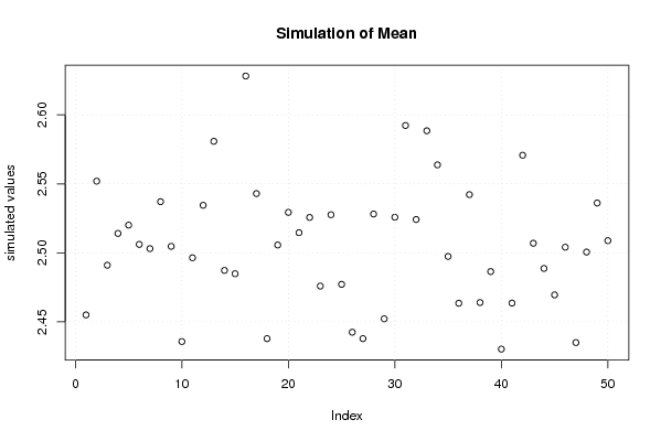
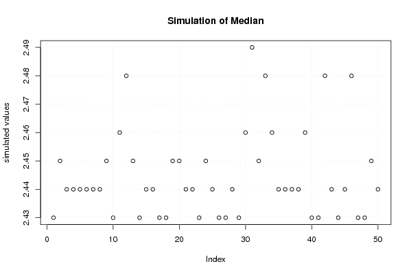
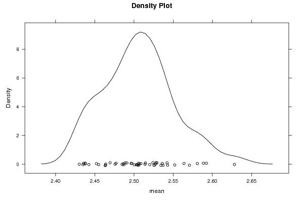
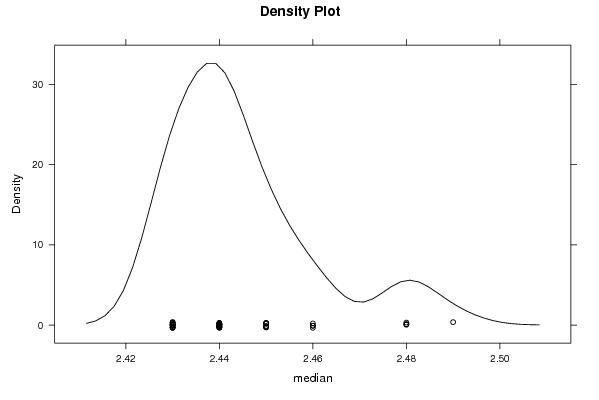
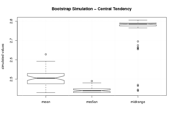
Title produced by software

Blocked Bootstrap Plot - Central Tendency

Date of computation

Wed, 16 Dec 2009 12:47:14 -0700

Cite this page as follows

Statistical Computations at FreeStatistics.org, Office for Research Development and Education, URL https://freestatistics.org/blog/index.php?v=date/2009/Dec/16/t1260992920ap6ske1y4u0sk2j.htm/, Retrieved Tue, 30 Apr 2024 15:50:03 +0000

Statistical Computations at FreeStatistics.org, Office for Research Development and Education, URL https://freestatistics.org/blog/index.php?pk=68578, Retrieved Tue, 30 Apr 2024 15:50:03 +0000

QR Codes:

Paste this QR Code to cite your computation.

Original text written by user:

IsPrivate?

No (this computation is public)

User-defined keywords

KDGP2W32

Estimated Impact

114

Family? (F = Feedback message, R = changed R code, M = changed R Module, P = changed Parameters, D = changed Data)

-       [Blocked Bootstrap Plot - Central Tendency] [Blocker Bootstrap...] [2009-12-16 19:47:14] [93f7fd88d04bfc03ecae616214d88989] [Current]

Feedback Forum

Post a new message

Dataseries X:

Download CSV

Histogram

Boxplots

2,46
2,46
2,45
2,45
2,46
2,43
2,44
2,44
2,43
2,43
2,42
2,43
2,43
2,42
2,41
2,42
2,39
2,4
2,39
2,4
2,41
2,41
2,41
2,41
2,42
2,43
2,43
2,43
2,44
2,42
2,44
2,42
2,42
2,42
2,43
2,44
2,43
2,44
2,44
2,45
2,45
2,43
2,44
2,45
2,46
2,44
2,43
2,42
2,41
2,43
2,41
2,43
2,43
2,44
2,43
2,44
2,43
2,44
2,44
2,43
2,43
2,43
2,43
2,44
2,47
2,48
2,49
2,5
2,51
2,49
2,49
2,48
2,48
2,48
2,5
2,5
2,5
2,5
2,5
2,48
2,49
2,48
2,5
2,5
2,49
2,48
2,47
2,46
2,43
2,42
2,43
2,45
2,45
2,46
2,44
2,45
2,45
2,42
2,41
2,39
2,39
2,38
2,37
2,37
2,38
2,39
2,41
2,42
2,48
2,53
2,56
2,56
2,53
2,57
2,56
2,57
2,58
2,57
2,6
2,63
2,72
2,83
2,9
2,92
2,94
2,95
2,98
3,02
3,16
3,2
3,18
3,17
3,19

Summary of computational transaction
Raw Input	view raw input (R code)
Raw Output	view raw output of R engine
Computing time	2 seconds
R Server	'Gwilym Jenkins' @ 72.249.127.135

\begin{tabular}{lllllllll}
\hline
Summary of computational transaction \tabularnewline
Raw Input & view raw input (R code)  \tabularnewline
Raw Output & view raw output of R engine  \tabularnewline
Computing time & 2 seconds \tabularnewline
R Server & 'Gwilym Jenkins' @ 72.249.127.135 \tabularnewline
\hline
\end{tabular}
%Source: https://freestatistics.org/blog/index.php?pk=68578&T=0

[TABLE]
[ROW][C]Summary of computational transaction[/C][/ROW]
[ROW][C]Raw Input[/C][C]view raw input (R code) [/C][/ROW]
[ROW][C]Raw Output[/C][C]view raw output of R engine [/C][/ROW]
[ROW][C]Computing time[/C][C]2 seconds[/C][/ROW]
[ROW][C]R Server[/C][C]'Gwilym Jenkins' @ 72.249.127.135[/C][/ROW]
[/TABLE]
Source: https://freestatistics.org/blog/index.php?pk=68578&T=0

Globally Unique Identifier (entire table): ba.freestatistics.org/blog/index.php?pk=68578&T=0

As an alternative you can also use a QR Code:

The GUIDs for individual cells are displayed in the table below:

Summary of computational transaction
Raw Input	view raw input (R code)
Raw Output	view raw output of R engine
Computing time	2 seconds
R Server	'Gwilym Jenkins' @ 72.249.127.135

Estimation Results of Blocked Bootstrap
statistic	Q1	Estimate	Q3	S.D.	IQR
mean	2.47618421052632	2.50706766917293	2.52902255639098	0.0446652206554154	0.0528383458646617
median	2.43	2.44	2.45	0.0154140142965645	0.02
midrange	2.77625	2.785	2.79	0.105314155879309	0.0137499999999999

\begin{tabular}{lllllllll}
\hline
Estimation Results of Blocked Bootstrap \tabularnewline
statistic & Q1 & Estimate & Q3 & S.D. & IQR \tabularnewline
mean & 2.47618421052632 & 2.50706766917293 & 2.52902255639098 & 0.0446652206554154 & 0.0528383458646617 \tabularnewline
median & 2.43 & 2.44 & 2.45 & 0.0154140142965645 & 0.02 \tabularnewline
midrange & 2.77625 & 2.785 & 2.79 & 0.105314155879309 & 0.0137499999999999 \tabularnewline
\hline
\end{tabular}
%Source: https://freestatistics.org/blog/index.php?pk=68578&T=1

[TABLE]
[ROW][C]Estimation Results of Blocked Bootstrap[/C][/ROW]
[ROW][C]statistic[/C][C]Q1[/C][C]Estimate[/C][C]Q3[/C][C]S.D.[/C][C]IQR[/C][/ROW]
[ROW][C]mean[/C][C]2.47618421052632[/C][C]2.50706766917293[/C][C]2.52902255639098[/C][C]0.0446652206554154[/C][C]0.0528383458646617[/C][/ROW]
[ROW][C]median[/C][C]2.43[/C][C]2.44[/C][C]2.45[/C][C]0.0154140142965645[/C][C]0.02[/C][/ROW]
[ROW][C]midrange[/C][C]2.77625[/C][C]2.785[/C][C]2.79[/C][C]0.105314155879309[/C][C]0.0137499999999999[/C][/ROW]
[/TABLE]
Source: https://freestatistics.org/blog/index.php?pk=68578&T=1

Globally Unique Identifier (entire table): ba.freestatistics.org/blog/index.php?pk=68578&T=1

As an alternative you can also use a QR Code:

The GUIDs for individual cells are displayed in the table below:

Estimation Results of Blocked Bootstrap
statistic	Q1	Estimate	Q3	S.D.	IQR
mean	2.47618421052632	2.50706766917293	2.52902255639098	0.0446652206554154	0.0528383458646617
median	2.43	2.44	2.45	0.0154140142965645	0.02
midrange	2.77625	2.785	2.79	0.105314155879309	0.0137499999999999

Figure 1

PNG link

Postscript link

PDF link

Figure 2

PNG link

Postscript link

PDF link

Figure 3

PNG link

Postscript link

PDF link

Figure 4

PNG link

Postscript link

PDF link

Figure 5

PNG link

Postscript link

PDF link

Figure 6

PNG link

Postscript link

PDF link

Figure 7

PNG link

Postscript link

PDF link

Parameters (Session):

par1 = 50 ; par2 = 12 ;

Parameters (R input):

par1 = 50 ; par2 = 12 ;

R code (references can be found in the software module):

par1 <- as.numeric(par1)
par2 <- as.numeric(par2)
if (par1 < 10) par1 = 10
if (par1 > 5000) par1 = 5000
if (par2 < 3) par2 = 3
if (par2 > length(x)) par2 = length(x)
library(lattice)
library(boot)
boot.stat <- function(s)
{
s.mean <- mean(s)
s.median <- median(s)
s.midrange <- (max(s) + min(s)) / 2
c(s.mean, s.median, s.midrange)
}
(r <- tsboot(x, boot.stat, R=par1, l=12, sim='fixed'))
bitmap(file='plot1.png')
plot(r$t[,1],type='p',ylab='simulated values',main='Simulation of Mean')
grid()
dev.off()
bitmap(file='plot2.png')
plot(r$t[,2],type='p',ylab='simulated values',main='Simulation of Median')
grid()
dev.off()
bitmap(file='plot3.png')
plot(r$t[,3],type='p',ylab='simulated values',main='Simulation of Midrange')
grid()
dev.off()
bitmap(file='plot4.png')
densityplot(~r$t[,1],col='black',main='Density Plot',xlab='mean')
dev.off()
bitmap(file='plot5.png')
densityplot(~r$t[,2],col='black',main='Density Plot',xlab='median')
dev.off()
bitmap(file='plot6.png')
densityplot(~r$t[,3],col='black',main='Density Plot',xlab='midrange')
dev.off()
z <- data.frame(cbind(r$t[,1],r$t[,2],r$t[,3]))
colnames(z) <- list('mean','median','midrange')
bitmap(file='plot7.png')
boxplot(z,notch=TRUE,ylab='simulated values',main='Bootstrap Simulation - Central Tendency')
grid()
dev.off()
load(file='createtable')
a<-table.start()
a<-table.row.start(a)
a<-table.element(a,'Estimation Results of Blocked Bootstrap',6,TRUE)
a<-table.row.end(a)
a<-table.row.start(a)
a<-table.element(a,'statistic',header=TRUE)
a<-table.element(a,'Q1',header=TRUE)
a<-table.element(a,'Estimate',header=TRUE)
a<-table.element(a,'Q3',header=TRUE)
a<-table.element(a,'S.D.',header=TRUE)
a<-table.element(a,'IQR',header=TRUE)
a<-table.row.end(a)
a<-table.row.start(a)
a<-table.element(a,'mean',header=TRUE)
q1 <- quantile(r$t[,1],0.25)[[1]]
q3 <- quantile(r$t[,1],0.75)[[1]]
a<-table.element(a,q1)
a<-table.element(a,r$t0[1])
a<-table.element(a,q3)
a<-table.element(a,sqrt(var(r$t[,1])))
a<-table.element(a,q3-q1)
a<-table.row.end(a)
a<-table.row.start(a)
a<-table.element(a,'median',header=TRUE)
q1 <- quantile(r$t[,2],0.25)[[1]]
q3 <- quantile(r$t[,2],0.75)[[1]]
a<-table.element(a,q1)
a<-table.element(a,r$t0[2])
a<-table.element(a,q3)
a<-table.element(a,sqrt(var(r$t[,2])))
a<-table.element(a,q3-q1)
a<-table.row.end(a)
a<-table.row.start(a)
a<-table.element(a,'midrange',header=TRUE)
q1 <- quantile(r$t[,3],0.25)[[1]]
q3 <- quantile(r$t[,3],0.75)[[1]]
a<-table.element(a,q1)
a<-table.element(a,r$t0[3])
a<-table.element(a,q3)
a<-table.element(a,sqrt(var(r$t[,3])))
a<-table.element(a,q3-q1)
a<-table.row.end(a)
a<-table.end(a)
table.save(a,file='mytable.tab')

Free Statistics

Description of Statistical Computation

Tree of Dependent Computations

Dataset

Tables (Output of Computation)

Figures (Output of Computation)

Input Parameters & R Code