Free Statistics
of Irreproducible Research!
Description of Statistical Computation | |||||||||||||||||||||
|---|---|---|---|---|---|---|---|---|---|---|---|---|---|---|---|---|---|---|---|---|---|
| Author's title | |||||||||||||||||||||
| Author | *The author of this computation has been verified* | ||||||||||||||||||||
| R Software Module | rwasp_cloud.wasp | ||||||||||||||||||||
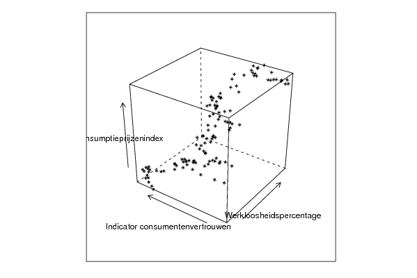
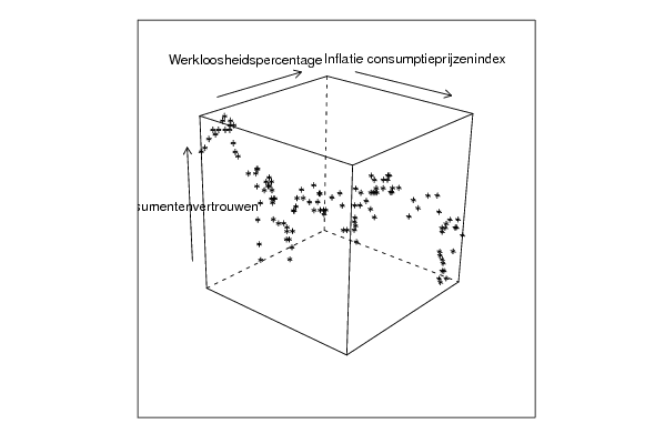
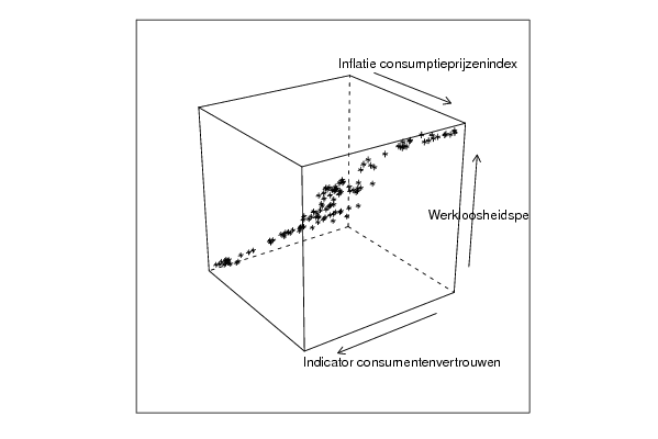
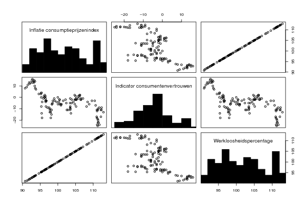
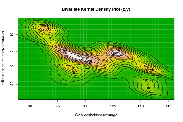
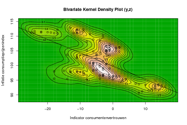
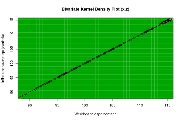
| Title produced by software | Trivariate Scatterplots | ||||||||||||||||||||
| Date of computation | Wed, 16 Dec 2009 08:48:39 -0700 | ||||||||||||||||||||
| Cite this page as follows | Statistical Computations at FreeStatistics.org, Office for Research Development and Education, URL https://freestatistics.org/blog/index.php?v=date/2009/Dec/16/t12609785924ew77avys5ho1qg.htm/, Retrieved Tue, 30 Apr 2024 19:05:32 +0000 | ||||||||||||||||||||
| Statistical Computations at FreeStatistics.org, Office for Research Development and Education, URL https://freestatistics.org/blog/index.php?pk=68438, Retrieved Tue, 30 Apr 2024 19:05:32 +0000 | |||||||||||||||||||||
| QR Codes: | |||||||||||||||||||||
|
| |||||||||||||||||||||
| Original text written by user: | |||||||||||||||||||||
| IsPrivate? | No (this computation is public) | ||||||||||||||||||||
| User-defined keywords | |||||||||||||||||||||
| Estimated Impact | 97 | ||||||||||||||||||||
Tree of Dependent Computations | |||||||||||||||||||||
| Family? (F = Feedback message, R = changed R code, M = changed R Module, P = changed Parameters, D = changed Data) | |||||||||||||||||||||
| - [Bivariate Kernel Density Estimation] [Bivariate kernel ...] [2009-12-15 10:15:21] [b458cdfea59edb592ddaf846f3f56c20] - RMPD [Trivariate Scatterplots] [] [2009-12-16 15:48:39] [95223d06eb2c638c714cd6fbd03e9e6c] [Current] | |||||||||||||||||||||
| Feedback Forum | |||||||||||||||||||||
Post a new message | |||||||||||||||||||||
Dataset | |||||||||||||||||||||
| Dataseries X: | |||||||||||||||||||||
91.02 91.19 91.53 91.88 92.06 92.32 92.67 92.85 92.82 93.46 93.23 93.54 93.29 93.20 93.60 93.81 94.62 95.22 95.38 95.31 95.30 95.57 95.42 95.53 95.33 95.90 96.06 96.31 96.34 96.49 96.22 96.53 96.50 96.77 96.66 96.58 96.63 97.06 97.73 98.01 97.76 97.49 97.77 97.96 98.23 98.51 98.19 98.37 98.31 98.60 98.97 99.11 99.64 100.03 99.98 100.32 100.44 100.51 101.00 100.88 100.55 100.83 101.51 102.16 102.39 102.54 102.85 103.47 103.57 103.69 103.50 103.47 103.45 103.48 103.93 103.89 104.40 104.79 104.77 105.13 105.26 104.96 104.75 105.01 105.15 105.20 105.77 105.78 106.26 106.13 106.12 106.57 106.44 106.54 107.10 108.10 108.40 108.84 109.62 110.42 110.67 111.66 112.28 112.87 112.18 112.36 112.16 111.49 111.25 111.36 111.74 111.10 111.33 111.25 111.04 110.97 111.31 111.02 111.07 111.36 | |||||||||||||||||||||
| Dataseries Y: | |||||||||||||||||||||
8 9 11 13 12 13 15 13 16 10 14 14 15 13 8 7 3 3 4 4 0 -4 -14 -18 -8 -1 1 2 0 1 0 -1 -3 -3 -3 -4 -8 -9 -13 -18 -11 -9 -10 -13 -11 -5 -15 -6 -6 -3 -1 -3 -4 -6 0 -4 -2 -2 -6 -7 -6 -6 -3 -2 -5 -11 -11 -11 -10 -14 -8 -9 -5 -1 -2 -5 -4 -6 -2 -2 -2 -2 2 1 -8 -1 1 -1 2 2 1 -1 -2 -2 -1 -8 -4 -6 -3 -3 -7 -9 -11 -13 -11 -9 -17 -22 -25 -20 -24 -24 -22 -19 -18 -17 -11 -11 -12 -10 | |||||||||||||||||||||
| Dataseries Z: | |||||||||||||||||||||
90.73 91.19 91.53 91.88 92.06 92.32 92.67 92.85 92.82 93.46 93.23 93.54 93.29 93.2 93.6 93.81 94.62 95.22 95.38 95.31 95.3 95.57 95.42 95.53 95.33 95.90 96.06 96.31 96.34 96.49 96.22 96.53 96.50 96.77 96.66 96.58 96.63 97.06 97.73 98.01 97.76 97.49 97.77 97.96 98.23 98.51 98.19 98.37 98.31 98.60 98.97 99.11 99.64 100.03 99.98 100.32 100.44 100.51 101.00 100.88 100.55 100.83 101.51 102.16 102.39 102.54 102.85 103.47 103.57 103.69 103.5 103.47 103.45 103.48 103.93 103.89 104.4 104.79 104.77 105.13 105.26 104.96 104.75 105.01 105.15 105.2 105.77 105.78 106.26 106.13 106.12 106.57 106.44 106.54 107.1 108.1 108.4 108.84 109.62 110.42 110.67 111.66 112.28 112.87 112.18 112.36 112.16 111.49 111.25 111.36 111.74 111.1 111.33 111.25 111.04 110.97 111.31 111.02 111.07 111.36 | |||||||||||||||||||||
Tables (Output of Computation) | |||||||||||||||||||||
| |||||||||||||||||||||
Figures (Output of Computation) | |||||||||||||||||||||
Input Parameters & R Code | |||||||||||||||||||||
| Parameters (Session): | |||||||||||||||||||||
| par1 = 50 ; par2 = 50 ; par3 = Y ; par4 = Y ; par5 = Werkloosheidspercentage ; par6 = Indicator consumentenvertrouwen ; par7 = Inflatie consumptieprijzenindex ; | |||||||||||||||||||||
| Parameters (R input): | |||||||||||||||||||||
| par1 = 50 ; par2 = 50 ; par3 = Y ; par4 = Y ; par5 = Werkloosheidspercentage ; par6 = Indicator consumentenvertrouwen ; par7 = Inflatie consumptieprijzenindex ; | |||||||||||||||||||||
| R code (references can be found in the software module): | |||||||||||||||||||||
x <- array(x,dim=c(length(x),1)) | |||||||||||||||||||||