Repository of Reproducible Computations

Free Statistics

of Irreproducible Research!

Author's title

Author

*The author of this computation has been verified*

R Software Module

rwasp_autocorrelation.wasp

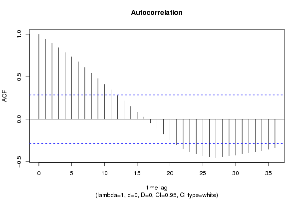
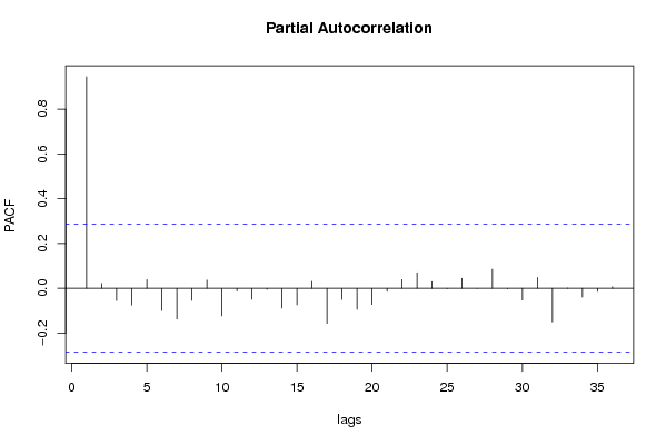
Title produced by software

(Partial) Autocorrelation Function

Date of computation

Tue, 15 Dec 2009 17:35:46 -0700

Cite this page as follows

Statistical Computations at FreeStatistics.org, Office for Research Development and Education, URL https://freestatistics.org/blog/index.php?v=date/2009/Dec/16/t1260923797mlqc02jf5j8vuws.htm/, Retrieved Tue, 30 Apr 2024 08:50:52 +0000

Statistical Computations at FreeStatistics.org, Office for Research Development and Education, URL https://freestatistics.org/blog/index.php?pk=68201, Retrieved Tue, 30 Apr 2024 08:50:52 +0000

QR Codes:

Paste this QR Code to cite your computation.

Original text written by user:

IsPrivate?

No (this computation is public)

User-defined keywords

Estimated Impact

145

Family? (F = Feedback message, R = changed R code, M = changed R Module, P = changed Parameters, D = changed Data)

-     [Univariate Explorative Data Analysis] [Run Sequence gebo...] [2008-12-12 13:32:37] [76963dc1903f0f612b6153510a3818cf]
- R  D  [Univariate Explorative Data Analysis] [Run Sequence gebo...] [2008-12-17 12:14:40] [76963dc1903f0f612b6153510a3818cf]
-         [Univariate Explorative Data Analysis] [Run Sequence Plot...] [2008-12-22 18:19:51] [1ce0d16c8f4225c977b42c8fa93bc163]
- RMP       [(Partial) Autocorrelation Function] [Identifying Integ...] [2009-11-22 12:16:10] [b98453cac15ba1066b407e146608df68]
-   PD        [(Partial) Autocorrelation Function] [Shwws8_v1] [2009-11-27 19:01:50] [5f89c040fdf1f8599c99d7f78a662321]
-   PD            [(Partial) Autocorrelation Function] [Paper] [2009-12-16 00:35:46] [93b66894f6318f3da4fcda772f2ffa6f] [Current]
-    D              [(Partial) Autocorrelation Function] [Paper] [2009-12-16 00:42:44] [5f89c040fdf1f8599c99d7f78a662321] 
-   PD                [(Partial) Autocorrelation Function] [] [2009-12-16 13:33:00] [5f89c040fdf1f8599c99d7f78a662321] 

Feedback Forum

Post a new message

Dataseries X:

Download CSV

Histogram

Boxplots

Summary of computational transaction
Raw Input	view raw input (R code)
Raw Output	view raw output of R engine
Computing time	2 seconds
R Server	'Gwilym Jenkins' @ 72.249.127.135

\begin{tabular}{lllllllll}
\hline
Summary of computational transaction \tabularnewline
Raw Input & view raw input (R code)  \tabularnewline
Raw Output & view raw output of R engine  \tabularnewline
Computing time & 2 seconds \tabularnewline
R Server & 'Gwilym Jenkins' @ 72.249.127.135 \tabularnewline
\hline
\end{tabular}
%Source: https://freestatistics.org/blog/index.php?pk=68201&T=0

[TABLE]
[ROW][C]Summary of computational transaction[/C][/ROW]
[ROW][C]Raw Input[/C][C]view raw input (R code) [/C][/ROW]
[ROW][C]Raw Output[/C][C]view raw output of R engine [/C][/ROW]
[ROW][C]Computing time[/C][C]2 seconds[/C][/ROW]
[ROW][C]R Server[/C][C]'Gwilym Jenkins' @ 72.249.127.135[/C][/ROW]
[/TABLE]
Source: https://freestatistics.org/blog/index.php?pk=68201&T=0

Globally Unique Identifier (entire table): ba.freestatistics.org/blog/index.php?pk=68201&T=0

As an alternative you can also use a QR Code:

The GUIDs for individual cells are displayed in the table below:

Summary of computational transaction
Raw Input	view raw input (R code)
Raw Output	view raw output of R engine
Computing time	2 seconds
R Server	'Gwilym Jenkins' @ 72.249.127.135

Autocorrelation Function
Time lag k	ACF(k)	T-STAT	P-value
1	0.945144	6.4796	0
2	0.895584	6.1398	0
3	0.84271	5.7773	0
4	0.785194	5.383	1e-06
5	0.735497	5.0423	4e-06
6	0.67733	4.6435	1.4e-05
7	0.609316	4.1773	6.3e-05
8	0.541256	3.7107	0.000273
9	0.479894	3.29	0.000952
10	0.409736	2.809	0.003609
11	0.345694	2.37	0.010973
12	0.27965	1.9172	0.030652
13	0.216106	1.4815	0.072567
14	0.151184	1.0365	0.152644
15	0.084192	0.5772	0.283282
16	0.026071	0.1787	0.429457
17	-0.043363	-0.2973	0.38378
18	-0.107268	-0.7354	0.232878
19	-0.174416	-1.1957	0.118899
20	-0.242118	-1.6599	0.051799
21	-0.300422	-2.0596	0.0225
22	-0.347288	-2.3809	0.010688
23	-0.382582	-2.6229	0.005859
24	-0.409948	-2.8105	0.003595
25	-0.430727	-2.9529	0.002451
26	-0.445331	-3.053	0.001861
27	-0.452308	-3.1009	0.001629
28	-0.445745	-3.0559	0.001846
29	-0.434535	-2.979	0.002282
30	-0.424751	-2.9119	0.002739
31	-0.406432	-2.7864	0.003832
32	-0.398652	-2.733	0.004408
33	-0.386274	-2.6482	0.005491
34	-0.370915	-2.5429	0.007173
35	-0.355343	-2.4361	0.009345
36	-0.335263	-2.2985	0.013015

\begin{tabular}{lllllllll}
\hline
Autocorrelation Function \tabularnewline
Time lag k & ACF(k) & T-STAT & P-value \tabularnewline
1 & 0.945144 & 6.4796 & 0 \tabularnewline
2 & 0.895584 & 6.1398 & 0 \tabularnewline
3 & 0.84271 & 5.7773 & 0 \tabularnewline
4 & 0.785194 & 5.383 & 1e-06 \tabularnewline
5 & 0.735497 & 5.0423 & 4e-06 \tabularnewline
6 & 0.67733 & 4.6435 & 1.4e-05 \tabularnewline
7 & 0.609316 & 4.1773 & 6.3e-05 \tabularnewline
8 & 0.541256 & 3.7107 & 0.000273 \tabularnewline
9 & 0.479894 & 3.29 & 0.000952 \tabularnewline
10 & 0.409736 & 2.809 & 0.003609 \tabularnewline
11 & 0.345694 & 2.37 & 0.010973 \tabularnewline
12 & 0.27965 & 1.9172 & 0.030652 \tabularnewline
13 & 0.216106 & 1.4815 & 0.072567 \tabularnewline
14 & 0.151184 & 1.0365 & 0.152644 \tabularnewline
15 & 0.084192 & 0.5772 & 0.283282 \tabularnewline
16 & 0.026071 & 0.1787 & 0.429457 \tabularnewline
17 & -0.043363 & -0.2973 & 0.38378 \tabularnewline
18 & -0.107268 & -0.7354 & 0.232878 \tabularnewline
19 & -0.174416 & -1.1957 & 0.118899 \tabularnewline
20 & -0.242118 & -1.6599 & 0.051799 \tabularnewline
21 & -0.300422 & -2.0596 & 0.0225 \tabularnewline
22 & -0.347288 & -2.3809 & 0.010688 \tabularnewline
23 & -0.382582 & -2.6229 & 0.005859 \tabularnewline
24 & -0.409948 & -2.8105 & 0.003595 \tabularnewline
25 & -0.430727 & -2.9529 & 0.002451 \tabularnewline
26 & -0.445331 & -3.053 & 0.001861 \tabularnewline
27 & -0.452308 & -3.1009 & 0.001629 \tabularnewline
28 & -0.445745 & -3.0559 & 0.001846 \tabularnewline
29 & -0.434535 & -2.979 & 0.002282 \tabularnewline
30 & -0.424751 & -2.9119 & 0.002739 \tabularnewline
31 & -0.406432 & -2.7864 & 0.003832 \tabularnewline
32 & -0.398652 & -2.733 & 0.004408 \tabularnewline
33 & -0.386274 & -2.6482 & 0.005491 \tabularnewline
34 & -0.370915 & -2.5429 & 0.007173 \tabularnewline
35 & -0.355343 & -2.4361 & 0.009345 \tabularnewline
36 & -0.335263 & -2.2985 & 0.013015 \tabularnewline
\hline
\end{tabular}
%Source: https://freestatistics.org/blog/index.php?pk=68201&T=1

[TABLE]
[ROW][C]Autocorrelation Function[/C][/ROW]
[ROW][C]Time lag k[/C][C]ACF(k)[/C][C]T-STAT[/C][C]P-value[/C][/ROW]
[ROW][C]1[/C][C]0.945144[/C][C]6.4796[/C][C]0[/C][/ROW]
[ROW][C]2[/C][C]0.895584[/C][C]6.1398[/C][C]0[/C][/ROW]
[ROW][C]3[/C][C]0.84271[/C][C]5.7773[/C][C]0[/C][/ROW]
[ROW][C]4[/C][C]0.785194[/C][C]5.383[/C][C]1e-06[/C][/ROW]
[ROW][C]5[/C][C]0.735497[/C][C]5.0423[/C][C]4e-06[/C][/ROW]
[ROW][C]6[/C][C]0.67733[/C][C]4.6435[/C][C]1.4e-05[/C][/ROW]
[ROW][C]7[/C][C]0.609316[/C][C]4.1773[/C][C]6.3e-05[/C][/ROW]
[ROW][C]8[/C][C]0.541256[/C][C]3.7107[/C][C]0.000273[/C][/ROW]
[ROW][C]9[/C][C]0.479894[/C][C]3.29[/C][C]0.000952[/C][/ROW]
[ROW][C]10[/C][C]0.409736[/C][C]2.809[/C][C]0.003609[/C][/ROW]
[ROW][C]11[/C][C]0.345694[/C][C]2.37[/C][C]0.010973[/C][/ROW]
[ROW][C]12[/C][C]0.27965[/C][C]1.9172[/C][C]0.030652[/C][/ROW]
[ROW][C]13[/C][C]0.216106[/C][C]1.4815[/C][C]0.072567[/C][/ROW]
[ROW][C]14[/C][C]0.151184[/C][C]1.0365[/C][C]0.152644[/C][/ROW]
[ROW][C]15[/C][C]0.084192[/C][C]0.5772[/C][C]0.283282[/C][/ROW]
[ROW][C]16[/C][C]0.026071[/C][C]0.1787[/C][C]0.429457[/C][/ROW]
[ROW][C]17[/C][C]-0.043363[/C][C]-0.2973[/C][C]0.38378[/C][/ROW]
[ROW][C]18[/C][C]-0.107268[/C][C]-0.7354[/C][C]0.232878[/C][/ROW]
[ROW][C]19[/C][C]-0.174416[/C][C]-1.1957[/C][C]0.118899[/C][/ROW]
[ROW][C]20[/C][C]-0.242118[/C][C]-1.6599[/C][C]0.051799[/C][/ROW]
[ROW][C]21[/C][C]-0.300422[/C][C]-2.0596[/C][C]0.0225[/C][/ROW]
[ROW][C]22[/C][C]-0.347288[/C][C]-2.3809[/C][C]0.010688[/C][/ROW]
[ROW][C]23[/C][C]-0.382582[/C][C]-2.6229[/C][C]0.005859[/C][/ROW]
[ROW][C]24[/C][C]-0.409948[/C][C]-2.8105[/C][C]0.003595[/C][/ROW]
[ROW][C]25[/C][C]-0.430727[/C][C]-2.9529[/C][C]0.002451[/C][/ROW]
[ROW][C]26[/C][C]-0.445331[/C][C]-3.053[/C][C]0.001861[/C][/ROW]
[ROW][C]27[/C][C]-0.452308[/C][C]-3.1009[/C][C]0.001629[/C][/ROW]
[ROW][C]28[/C][C]-0.445745[/C][C]-3.0559[/C][C]0.001846[/C][/ROW]
[ROW][C]29[/C][C]-0.434535[/C][C]-2.979[/C][C]0.002282[/C][/ROW]
[ROW][C]30[/C][C]-0.424751[/C][C]-2.9119[/C][C]0.002739[/C][/ROW]
[ROW][C]31[/C][C]-0.406432[/C][C]-2.7864[/C][C]0.003832[/C][/ROW]
[ROW][C]32[/C][C]-0.398652[/C][C]-2.733[/C][C]0.004408[/C][/ROW]
[ROW][C]33[/C][C]-0.386274[/C][C]-2.6482[/C][C]0.005491[/C][/ROW]
[ROW][C]34[/C][C]-0.370915[/C][C]-2.5429[/C][C]0.007173[/C][/ROW]
[ROW][C]35[/C][C]-0.355343[/C][C]-2.4361[/C][C]0.009345[/C][/ROW]
[ROW][C]36[/C][C]-0.335263[/C][C]-2.2985[/C][C]0.013015[/C][/ROW]
[/TABLE]
Source: https://freestatistics.org/blog/index.php?pk=68201&T=1

Globally Unique Identifier (entire table): ba.freestatistics.org/blog/index.php?pk=68201&T=1

As an alternative you can also use a QR Code:

The GUIDs for individual cells are displayed in the table below:

Autocorrelation Function
Time lag k	ACF(k)	T-STAT	P-value
1	0.945144	6.4796	0
2	0.895584	6.1398	0
3	0.84271	5.7773	0
4	0.785194	5.383	1e-06
5	0.735497	5.0423	4e-06
6	0.67733	4.6435	1.4e-05
7	0.609316	4.1773	6.3e-05
8	0.541256	3.7107	0.000273
9	0.479894	3.29	0.000952
10	0.409736	2.809	0.003609
11	0.345694	2.37	0.010973
12	0.27965	1.9172	0.030652
13	0.216106	1.4815	0.072567
14	0.151184	1.0365	0.152644
15	0.084192	0.5772	0.283282
16	0.026071	0.1787	0.429457
17	-0.043363	-0.2973	0.38378
18	-0.107268	-0.7354	0.232878
19	-0.174416	-1.1957	0.118899
20	-0.242118	-1.6599	0.051799
21	-0.300422	-2.0596	0.0225
22	-0.347288	-2.3809	0.010688
23	-0.382582	-2.6229	0.005859
24	-0.409948	-2.8105	0.003595
25	-0.430727	-2.9529	0.002451
26	-0.445331	-3.053	0.001861
27	-0.452308	-3.1009	0.001629
28	-0.445745	-3.0559	0.001846
29	-0.434535	-2.979	0.002282
30	-0.424751	-2.9119	0.002739
31	-0.406432	-2.7864	0.003832
32	-0.398652	-2.733	0.004408
33	-0.386274	-2.6482	0.005491
34	-0.370915	-2.5429	0.007173
35	-0.355343	-2.4361	0.009345
36	-0.335263	-2.2985	0.013015

Partial Autocorrelation Function
Time lag k	PACF(k)	T-STAT	P-value
1	0.945144	6.4796	0
2	0.021435	0.147	0.441899
3	-0.054947	-0.3767	0.354046
4	-0.075102	-0.5149	0.304527
5	0.038217	0.262	0.397233
6	-0.099714	-0.6836	0.248791
7	-0.137866	-0.9452	0.174704
8	-0.054555	-0.374	0.35504
9	0.036223	0.2483	0.40248
10	-0.12349	-0.8466	0.200752
11	-0.012138	-0.0832	0.467018
12	-0.049252	-0.3377	0.368564
13	-0.004635	-0.0318	0.487393
14	-0.088465	-0.6065	0.273555
15	-0.074517	-0.5109	0.305918
16	0.030903	0.2119	0.416565
17	-0.156635	-1.0738	0.144189
18	-0.050099	-0.3435	0.366391
19	-0.093948	-0.6441	0.261329
20	-0.072682	-0.4983	0.310304
21	-0.013086	-0.0897	0.464447
22	0.039073	0.2679	0.394986
23	0.069225	0.4746	0.31864
24	0.029329	0.2011	0.420757
25	-0.001661	-0.0114	0.495482
26	0.044466	0.3048	0.380915
27	-0.00098	-0.0067	0.497333
28	0.084953	0.5824	0.281538
29	-0.002259	-0.0155	0.493855
30	-0.052198	-0.3579	0.361027
31	0.048198	0.3304	0.371272
32	-0.14993	-1.0279	0.154636
33	0.000911	0.0062	0.497522
34	-0.039168	-0.2685	0.394735
35	-0.013724	-0.0941	0.46272
36	0.006483	0.0444	0.482368

\begin{tabular}{lllllllll}
\hline
Partial Autocorrelation Function \tabularnewline
Time lag k & PACF(k) & T-STAT & P-value \tabularnewline
1 & 0.945144 & 6.4796 & 0 \tabularnewline
2 & 0.021435 & 0.147 & 0.441899 \tabularnewline
3 & -0.054947 & -0.3767 & 0.354046 \tabularnewline
4 & -0.075102 & -0.5149 & 0.304527 \tabularnewline
5 & 0.038217 & 0.262 & 0.397233 \tabularnewline
6 & -0.099714 & -0.6836 & 0.248791 \tabularnewline
7 & -0.137866 & -0.9452 & 0.174704 \tabularnewline
8 & -0.054555 & -0.374 & 0.35504 \tabularnewline
9 & 0.036223 & 0.2483 & 0.40248 \tabularnewline
10 & -0.12349 & -0.8466 & 0.200752 \tabularnewline
11 & -0.012138 & -0.0832 & 0.467018 \tabularnewline
12 & -0.049252 & -0.3377 & 0.368564 \tabularnewline
13 & -0.004635 & -0.0318 & 0.487393 \tabularnewline
14 & -0.088465 & -0.6065 & 0.273555 \tabularnewline
15 & -0.074517 & -0.5109 & 0.305918 \tabularnewline
16 & 0.030903 & 0.2119 & 0.416565 \tabularnewline
17 & -0.156635 & -1.0738 & 0.144189 \tabularnewline
18 & -0.050099 & -0.3435 & 0.366391 \tabularnewline
19 & -0.093948 & -0.6441 & 0.261329 \tabularnewline
20 & -0.072682 & -0.4983 & 0.310304 \tabularnewline
21 & -0.013086 & -0.0897 & 0.464447 \tabularnewline
22 & 0.039073 & 0.2679 & 0.394986 \tabularnewline
23 & 0.069225 & 0.4746 & 0.31864 \tabularnewline
24 & 0.029329 & 0.2011 & 0.420757 \tabularnewline
25 & -0.001661 & -0.0114 & 0.495482 \tabularnewline
26 & 0.044466 & 0.3048 & 0.380915 \tabularnewline
27 & -0.00098 & -0.0067 & 0.497333 \tabularnewline
28 & 0.084953 & 0.5824 & 0.281538 \tabularnewline
29 & -0.002259 & -0.0155 & 0.493855 \tabularnewline
30 & -0.052198 & -0.3579 & 0.361027 \tabularnewline
31 & 0.048198 & 0.3304 & 0.371272 \tabularnewline
32 & -0.14993 & -1.0279 & 0.154636 \tabularnewline
33 & 0.000911 & 0.0062 & 0.497522 \tabularnewline
34 & -0.039168 & -0.2685 & 0.394735 \tabularnewline
35 & -0.013724 & -0.0941 & 0.46272 \tabularnewline
36 & 0.006483 & 0.0444 & 0.482368 \tabularnewline
\hline
\end{tabular}
%Source: https://freestatistics.org/blog/index.php?pk=68201&T=2

[TABLE]
[ROW][C]Partial Autocorrelation Function[/C][/ROW]
[ROW][C]Time lag k[/C][C]PACF(k)[/C][C]T-STAT[/C][C]P-value[/C][/ROW]
[ROW][C]1[/C][C]0.945144[/C][C]6.4796[/C][C]0[/C][/ROW]
[ROW][C]2[/C][C]0.021435[/C][C]0.147[/C][C]0.441899[/C][/ROW]
[ROW][C]3[/C][C]-0.054947[/C][C]-0.3767[/C][C]0.354046[/C][/ROW]
[ROW][C]4[/C][C]-0.075102[/C][C]-0.5149[/C][C]0.304527[/C][/ROW]
[ROW][C]5[/C][C]0.038217[/C][C]0.262[/C][C]0.397233[/C][/ROW]
[ROW][C]6[/C][C]-0.099714[/C][C]-0.6836[/C][C]0.248791[/C][/ROW]
[ROW][C]7[/C][C]-0.137866[/C][C]-0.9452[/C][C]0.174704[/C][/ROW]
[ROW][C]8[/C][C]-0.054555[/C][C]-0.374[/C][C]0.35504[/C][/ROW]
[ROW][C]9[/C][C]0.036223[/C][C]0.2483[/C][C]0.40248[/C][/ROW]
[ROW][C]10[/C][C]-0.12349[/C][C]-0.8466[/C][C]0.200752[/C][/ROW]
[ROW][C]11[/C][C]-0.012138[/C][C]-0.0832[/C][C]0.467018[/C][/ROW]
[ROW][C]12[/C][C]-0.049252[/C][C]-0.3377[/C][C]0.368564[/C][/ROW]
[ROW][C]13[/C][C]-0.004635[/C][C]-0.0318[/C][C]0.487393[/C][/ROW]
[ROW][C]14[/C][C]-0.088465[/C][C]-0.6065[/C][C]0.273555[/C][/ROW]
[ROW][C]15[/C][C]-0.074517[/C][C]-0.5109[/C][C]0.305918[/C][/ROW]
[ROW][C]16[/C][C]0.030903[/C][C]0.2119[/C][C]0.416565[/C][/ROW]
[ROW][C]17[/C][C]-0.156635[/C][C]-1.0738[/C][C]0.144189[/C][/ROW]
[ROW][C]18[/C][C]-0.050099[/C][C]-0.3435[/C][C]0.366391[/C][/ROW]
[ROW][C]19[/C][C]-0.093948[/C][C]-0.6441[/C][C]0.261329[/C][/ROW]
[ROW][C]20[/C][C]-0.072682[/C][C]-0.4983[/C][C]0.310304[/C][/ROW]
[ROW][C]21[/C][C]-0.013086[/C][C]-0.0897[/C][C]0.464447[/C][/ROW]
[ROW][C]22[/C][C]0.039073[/C][C]0.2679[/C][C]0.394986[/C][/ROW]
[ROW][C]23[/C][C]0.069225[/C][C]0.4746[/C][C]0.31864[/C][/ROW]
[ROW][C]24[/C][C]0.029329[/C][C]0.2011[/C][C]0.420757[/C][/ROW]
[ROW][C]25[/C][C]-0.001661[/C][C]-0.0114[/C][C]0.495482[/C][/ROW]
[ROW][C]26[/C][C]0.044466[/C][C]0.3048[/C][C]0.380915[/C][/ROW]
[ROW][C]27[/C][C]-0.00098[/C][C]-0.0067[/C][C]0.497333[/C][/ROW]
[ROW][C]28[/C][C]0.084953[/C][C]0.5824[/C][C]0.281538[/C][/ROW]
[ROW][C]29[/C][C]-0.002259[/C][C]-0.0155[/C][C]0.493855[/C][/ROW]
[ROW][C]30[/C][C]-0.052198[/C][C]-0.3579[/C][C]0.361027[/C][/ROW]
[ROW][C]31[/C][C]0.048198[/C][C]0.3304[/C][C]0.371272[/C][/ROW]
[ROW][C]32[/C][C]-0.14993[/C][C]-1.0279[/C][C]0.154636[/C][/ROW]
[ROW][C]33[/C][C]0.000911[/C][C]0.0062[/C][C]0.497522[/C][/ROW]
[ROW][C]34[/C][C]-0.039168[/C][C]-0.2685[/C][C]0.394735[/C][/ROW]
[ROW][C]35[/C][C]-0.013724[/C][C]-0.0941[/C][C]0.46272[/C][/ROW]
[ROW][C]36[/C][C]0.006483[/C][C]0.0444[/C][C]0.482368[/C][/ROW]
[/TABLE]
Source: https://freestatistics.org/blog/index.php?pk=68201&T=2

Globally Unique Identifier (entire table): ba.freestatistics.org/blog/index.php?pk=68201&T=2

As an alternative you can also use a QR Code:

The GUIDs for individual cells are displayed in the table below:

Partial Autocorrelation Function
Time lag k	PACF(k)	T-STAT	P-value
1	0.945144	6.4796	0
2	0.021435	0.147	0.441899
3	-0.054947	-0.3767	0.354046
4	-0.075102	-0.5149	0.304527
5	0.038217	0.262	0.397233
6	-0.099714	-0.6836	0.248791
7	-0.137866	-0.9452	0.174704
8	-0.054555	-0.374	0.35504
9	0.036223	0.2483	0.40248
10	-0.12349	-0.8466	0.200752
11	-0.012138	-0.0832	0.467018
12	-0.049252	-0.3377	0.368564
13	-0.004635	-0.0318	0.487393
14	-0.088465	-0.6065	0.273555
15	-0.074517	-0.5109	0.305918
16	0.030903	0.2119	0.416565
17	-0.156635	-1.0738	0.144189
18	-0.050099	-0.3435	0.366391
19	-0.093948	-0.6441	0.261329
20	-0.072682	-0.4983	0.310304
21	-0.013086	-0.0897	0.464447
22	0.039073	0.2679	0.394986
23	0.069225	0.4746	0.31864
24	0.029329	0.2011	0.420757
25	-0.001661	-0.0114	0.495482
26	0.044466	0.3048	0.380915
27	-0.00098	-0.0067	0.497333
28	0.084953	0.5824	0.281538
29	-0.002259	-0.0155	0.493855
30	-0.052198	-0.3579	0.361027
31	0.048198	0.3304	0.371272
32	-0.14993	-1.0279	0.154636
33	0.000911	0.0062	0.497522
34	-0.039168	-0.2685	0.394735
35	-0.013724	-0.0941	0.46272
36	0.006483	0.0444	0.482368

Figure 1

PNG link

Postscript link

PDF link

Figure 2

PNG link

Postscript link

PDF link

Parameters (Session):

par1 = 36 ; par2 = 1 ; par3 = 0 ; par4 = 0 ; par5 = 12 ; par6 = White Noise ; par7 = 0.95 ;

Parameters (R input):

par1 = 36 ; par2 = 1 ; par3 = 0 ; par4 = 0 ; par5 = 12 ; par6 = White Noise ; par7 = 0.95 ;

R code (references can be found in the software module):

if (par1 == 'Default') {
par1 = 10*log10(length(x))
} else {
par1 <- as.numeric(par1)
}
par2 <- as.numeric(par2)
par3 <- as.numeric(par3)
par4 <- as.numeric(par4)
par5 <- as.numeric(par5)
if (par6 == 'White Noise') par6 <- 'white' else par6 <- 'ma'
par7 <- as.numeric(par7)
if (par2 == 0) {
x <- log(x)
} else {
x <- (x ^ par2 - 1) / par2
}
if (par3 > 0) x <- diff(x,lag=1,difference=par3)
if (par4 > 0) x <- diff(x,lag=par5,difference=par4)
bitmap(file='pic1.png')
racf <- acf(x, par1, main='Autocorrelation', xlab='time lag', ylab='ACF', ci.type=par6, ci=par7, sub=paste('(lambda=',par2,', d=',par3,', D=',par4,', CI=', par7, ', CI type=',par6,')',sep=''))
dev.off()
bitmap(file='pic2.png')
rpacf <- pacf(x,par1,main='Partial Autocorrelation',xlab='lags',ylab='PACF')
dev.off()
(myacf <- c(racf$acf))
(mypacf <- c(rpacf$acf))
lengthx <- length(x)
sqrtn <- sqrt(lengthx)
load(file='createtable')
a<-table.start()
a<-table.row.start(a)
a<-table.element(a,'Autocorrelation Function',4,TRUE)
a<-table.row.end(a)
a<-table.row.start(a)
a<-table.element(a,'Time lag k',header=TRUE)
a<-table.element(a,hyperlink('basics.htm','ACF(k)','click here for more information about the Autocorrelation Function'),header=TRUE)
a<-table.element(a,'T-STAT',header=TRUE)
a<-table.element(a,'P-value',header=TRUE)
a<-table.row.end(a)
for (i in 2:(par1+1)) {
a<-table.row.start(a)
a<-table.element(a,i-1,header=TRUE)
a<-table.element(a,round(myacf[i],6))
mytstat <- myacf[i]*sqrtn
a<-table.element(a,round(mytstat,4))
a<-table.element(a,round(1-pt(abs(mytstat),lengthx),6))
a<-table.row.end(a)
}
a<-table.end(a)
table.save(a,file='mytable.tab')
a<-table.start()
a<-table.row.start(a)
a<-table.element(a,'Partial Autocorrelation Function',4,TRUE)
a<-table.row.end(a)
a<-table.row.start(a)
a<-table.element(a,'Time lag k',header=TRUE)
a<-table.element(a,hyperlink('basics.htm','PACF(k)','click here for more information about the Partial Autocorrelation Function'),header=TRUE)
a<-table.element(a,'T-STAT',header=TRUE)
a<-table.element(a,'P-value',header=TRUE)
a<-table.row.end(a)
for (i in 1:par1) {
a<-table.row.start(a)
a<-table.element(a,i,header=TRUE)
a<-table.element(a,round(mypacf[i],6))
mytstat <- mypacf[i]*sqrtn
a<-table.element(a,round(mytstat,4))
a<-table.element(a,round(1-pt(abs(mytstat),lengthx),6))
a<-table.row.end(a)
}
a<-table.end(a)
table.save(a,file='mytable1.tab')

Free Statistics

Description of Statistical Computation

Tree of Dependent Computations

Dataset

Tables (Output of Computation)

Figures (Output of Computation)

Input Parameters & R Code