Repository of Reproducible Computations

Free Statistics

of Irreproducible Research!

Author's title

Author

*The author of this computation has been verified*

R Software Module

rwasp_arimaforecasting.wasp

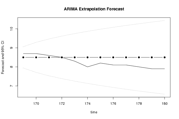
Title produced by software

ARIMA Forecasting

Date of computation

Sat, 12 Dec 2009 12:25:39 -0700

Cite this page as follows

Statistical Computations at FreeStatistics.org, Office for Research Development and Education, URL https://freestatistics.org/blog/index.php?v=date/2009/Dec/12/t1260646035oi7vorf8l9d05ec.htm/, Retrieved Mon, 29 Apr 2024 14:57:59 +0000

Statistical Computations at FreeStatistics.org, Office for Research Development and Education, URL https://freestatistics.org/blog/index.php?pk=67130, Retrieved Mon, 29 Apr 2024 14:57:59 +0000

QR Codes:

Paste this QR Code to cite your computation.

Original text written by user:

IsPrivate?

No (this computation is public)

User-defined keywords

workshop 10 review

Estimated Impact

157

Family? (F = Feedback message, R = changed R code, M = changed R Module, P = changed Parameters, D = changed Data)

-     [ARIMA Forecasting] [] [2009-12-07 09:54:52] [b98453cac15ba1066b407e146608df68]
- R PD  [ARIMA Forecasting] [workshop 10] [2009-12-09 18:40:24] [74be16979710d4c4e7c6647856088456]
-    D      [ARIMA Forecasting] [workshop 10 review] [2009-12-12 19:25:39] [6198946fb53eb5eb18db46bb758f7fde] [Current]
- R P         [ARIMA Forecasting] [paper] [2009-12-15 18:35:07] [3d8acb8ffdb376c5fec19e610f8198c2] 
-               [ARIMA Forecasting] [paper] [2009-12-22 20:01:15] [3d8acb8ffdb376c5fec19e610f8198c2] 
-               [ARIMA Forecasting] [paper] [2009-12-22 20:03:12] [3d8acb8ffdb376c5fec19e610f8198c2] 

Feedback Forum

Post a new message

Dataseries X:

Download CSV

Histogram

Boxplots

6.9
6.8
6.7
6.6
6.5
6.5
7.0
7.5
7.6
7.6
7.6
7.8
8.0
8.0
8.0
7.9
7.9
8.0
8.5
9.2
9.4
9.5
9.5
9.6
9.7
9.7
9.6
9.5
9.4
9.3
9.6
10.2
10.2
10.1
9.9
9.8
9.8
9.7
9.5
9.3
9.1
9.0
9.5
10.0
10.2
10.1
10.0
9.9
10.0
9.9
9.7
9.5
9.2
9.0
9.3
9.8
9.8
9.6
9.4
9.3
9.2
9.2
9.0
8.8
8.7
8.7
9.1
9.7
9.8
9.6
9.4
9.4
9.5
9.4
9.3
9.2
9.0
8.9
9.2
9.8
9.9
9.6
9.2
9.1
9.1
9.0
8.9
8.7
8.5
8.3
8.5
8.7
8.4
8.1
7.8
7.7
7.5
7.2
6.8
6.7
6.4
6.3
6.8
7.3
7.1
7.0
6.8
6.6
6.3
6.1
6.1
6.3
6.3
6.0
6.2
6.4
6.8
7.5
7.5
7.6
7.6
7.4
7.3
7.1
6.9
6.8
7.5
7.6
7.8
8.0
8.1
8.2
8.3
8.2
8.0
7.9
7.6
7.6
8.3
8.4
8.4
8.4
8.4
8.6
8.9
8.8
8.3
7.5
7.2
7.4
8.8
9.3
9.3
8.7
8.2
8.3
8.5
8.6
8.5
8.2
8.1
7.9
8.6
8.7
8.7
8.5
8.4
8.5
8.7
8.7
8.6
8.5
8.3
8.0
8.2
8.1
8.1
8.0
7.9
7.9

Summary of computational transaction
Raw Input	view raw input (R code)
Raw Output	view raw output of R engine
Computing time	1 seconds
R Server	'Gwilym Jenkins' @ 72.249.127.135

\begin{tabular}{lllllllll}
\hline
Summary of computational transaction \tabularnewline
Raw Input & view raw input (R code)  \tabularnewline
Raw Output & view raw output of R engine  \tabularnewline
Computing time & 1 seconds \tabularnewline
R Server & 'Gwilym Jenkins' @ 72.249.127.135 \tabularnewline
\hline
\end{tabular}
%Source: https://freestatistics.org/blog/index.php?pk=67130&T=0

[TABLE]
[ROW][C]Summary of computational transaction[/C][/ROW]
[ROW][C]Raw Input[/C][C]view raw input (R code) [/C][/ROW]
[ROW][C]Raw Output[/C][C]view raw output of R engine [/C][/ROW]
[ROW][C]Computing time[/C][C]1 seconds[/C][/ROW]
[ROW][C]R Server[/C][C]'Gwilym Jenkins' @ 72.249.127.135[/C][/ROW]
[/TABLE]
Source: https://freestatistics.org/blog/index.php?pk=67130&T=0

Globally Unique Identifier (entire table): ba.freestatistics.org/blog/index.php?pk=67130&T=0

As an alternative you can also use a QR Code:

The GUIDs for individual cells are displayed in the table below:

Summary of computational transaction
Raw Input	view raw input (R code)
Raw Output	view raw output of R engine
Computing time	1 seconds
R Server	'Gwilym Jenkins' @ 72.249.127.135

Univariate ARIMA Extrapolation Forecast
time	Y[t]	F[t]	95% LB	95% UB	p-value(H0: Y[t] = F[t])	P(F[t]>Y[t-1])	P(F[t]>Y[t-s])	P(F[t]>Y[168])
156	8.3	-	-	-	-	-	-	-
157	8.5	-	-	-	-	-	-	-
158	8.6	-	-	-	-	-	-	-
159	8.5	-	-	-	-	-	-	-
160	8.2	-	-	-	-	-	-	-
161	8.1	-	-	-	-	-	-	-
162	7.9	-	-	-	-	-	-	-
163	8.6	-	-	-	-	-	-	-
164	8.7	-	-	-	-	-	-	-
165	8.7	-	-	-	-	-	-	-
166	8.5	-	-	-	-	-	-	-
167	8.4	-	-	-	-	-	-	-
168	8.5	-	-	-	-	-	-	-
169	8.7	8.5	7.9411	9.0589	0.2415	0.5	0.5	0.5
170	8.7	8.5	7.7096	9.2904	0.31	0.31	0.4021	0.5
171	8.6	8.5	7.5319	9.4681	0.4198	0.3428	0.5	0.5
172	8.5	8.5	7.3822	9.6178	0.5	0.4304	0.7006	0.5
173	8.3	8.5	7.2502	9.7498	0.3769	0.5	0.7348	0.5
174	8	8.5	7.1309	9.8691	0.2371	0.6127	0.8048	0.5
175	8.2	8.5	7.0212	9.9788	0.3455	0.7462	0.4473	0.5
176	8.1	8.5	6.9191	10.0809	0.31	0.645	0.4021	0.5
177	8.1	8.5	6.8232	10.1768	0.32	0.68	0.4076	0.5
178	8	8.5	6.7325	10.2675	0.2896	0.6713	0.5	0.5
179	7.9	8.5	6.6463	10.3537	0.2629	0.7015	0.5421	0.5
180	7.9	8.5	6.5639	10.4361	0.2718	0.7282	0.5	0.5

\begin{tabular}{lllllllll}
\hline
Univariate ARIMA Extrapolation Forecast \tabularnewline
time & Y[t] & F[t] & 95% LB & 95% UB & p-value(H0: Y[t] = F[t]) & P(F[t]>Y[t-1]) & P(F[t]>Y[t-s]) & P(F[t]>Y[168]) \tabularnewline
156 & 8.3 & - & - & - & - & - & - & - \tabularnewline
157 & 8.5 & - & - & - & - & - & - & - \tabularnewline
158 & 8.6 & - & - & - & - & - & - & - \tabularnewline
159 & 8.5 & - & - & - & - & - & - & - \tabularnewline
160 & 8.2 & - & - & - & - & - & - & - \tabularnewline
161 & 8.1 & - & - & - & - & - & - & - \tabularnewline
162 & 7.9 & - & - & - & - & - & - & - \tabularnewline
163 & 8.6 & - & - & - & - & - & - & - \tabularnewline
164 & 8.7 & - & - & - & - & - & - & - \tabularnewline
165 & 8.7 & - & - & - & - & - & - & - \tabularnewline
166 & 8.5 & - & - & - & - & - & - & - \tabularnewline
167 & 8.4 & - & - & - & - & - & - & - \tabularnewline
168 & 8.5 & - & - & - & - & - & - & - \tabularnewline
169 & 8.7 & 8.5 & 7.9411 & 9.0589 & 0.2415 & 0.5 & 0.5 & 0.5 \tabularnewline
170 & 8.7 & 8.5 & 7.7096 & 9.2904 & 0.31 & 0.31 & 0.4021 & 0.5 \tabularnewline
171 & 8.6 & 8.5 & 7.5319 & 9.4681 & 0.4198 & 0.3428 & 0.5 & 0.5 \tabularnewline
172 & 8.5 & 8.5 & 7.3822 & 9.6178 & 0.5 & 0.4304 & 0.7006 & 0.5 \tabularnewline
173 & 8.3 & 8.5 & 7.2502 & 9.7498 & 0.3769 & 0.5 & 0.7348 & 0.5 \tabularnewline
174 & 8 & 8.5 & 7.1309 & 9.8691 & 0.2371 & 0.6127 & 0.8048 & 0.5 \tabularnewline
175 & 8.2 & 8.5 & 7.0212 & 9.9788 & 0.3455 & 0.7462 & 0.4473 & 0.5 \tabularnewline
176 & 8.1 & 8.5 & 6.9191 & 10.0809 & 0.31 & 0.645 & 0.4021 & 0.5 \tabularnewline
177 & 8.1 & 8.5 & 6.8232 & 10.1768 & 0.32 & 0.68 & 0.4076 & 0.5 \tabularnewline
178 & 8 & 8.5 & 6.7325 & 10.2675 & 0.2896 & 0.6713 & 0.5 & 0.5 \tabularnewline
179 & 7.9 & 8.5 & 6.6463 & 10.3537 & 0.2629 & 0.7015 & 0.5421 & 0.5 \tabularnewline
180 & 7.9 & 8.5 & 6.5639 & 10.4361 & 0.2718 & 0.7282 & 0.5 & 0.5 \tabularnewline
\hline
\end{tabular}
%Source: https://freestatistics.org/blog/index.php?pk=67130&T=1

[TABLE]
[ROW][C]Univariate ARIMA Extrapolation Forecast[/C][/ROW]
[ROW][C]time[/C][C]Y[t][/C][C]F[t][/C][C]95% LB[/C][C]95% UB[/C][C]p-value(H0: Y[t] = F[t])[/C][C]P(F[t]>Y[t-1])[/C][C]P(F[t]>Y[t-s])[/C][C]P(F[t]>Y[168])[/C][/ROW]
[ROW][C]156[/C][C]8.3[/C][C]-[/C][C]-[/C][C]-[/C][C]-[/C][C]-[/C][C]-[/C][C]-[/C][/ROW]
[ROW][C]157[/C][C]8.5[/C][C]-[/C][C]-[/C][C]-[/C][C]-[/C][C]-[/C][C]-[/C][C]-[/C][/ROW]
[ROW][C]158[/C][C]8.6[/C][C]-[/C][C]-[/C][C]-[/C][C]-[/C][C]-[/C][C]-[/C][C]-[/C][/ROW]
[ROW][C]159[/C][C]8.5[/C][C]-[/C][C]-[/C][C]-[/C][C]-[/C][C]-[/C][C]-[/C][C]-[/C][/ROW]
[ROW][C]160[/C][C]8.2[/C][C]-[/C][C]-[/C][C]-[/C][C]-[/C][C]-[/C][C]-[/C][C]-[/C][/ROW]
[ROW][C]161[/C][C]8.1[/C][C]-[/C][C]-[/C][C]-[/C][C]-[/C][C]-[/C][C]-[/C][C]-[/C][/ROW]
[ROW][C]162[/C][C]7.9[/C][C]-[/C][C]-[/C][C]-[/C][C]-[/C][C]-[/C][C]-[/C][C]-[/C][/ROW]
[ROW][C]163[/C][C]8.6[/C][C]-[/C][C]-[/C][C]-[/C][C]-[/C][C]-[/C][C]-[/C][C]-[/C][/ROW]
[ROW][C]164[/C][C]8.7[/C][C]-[/C][C]-[/C][C]-[/C][C]-[/C][C]-[/C][C]-[/C][C]-[/C][/ROW]
[ROW][C]165[/C][C]8.7[/C][C]-[/C][C]-[/C][C]-[/C][C]-[/C][C]-[/C][C]-[/C][C]-[/C][/ROW]
[ROW][C]166[/C][C]8.5[/C][C]-[/C][C]-[/C][C]-[/C][C]-[/C][C]-[/C][C]-[/C][C]-[/C][/ROW]
[ROW][C]167[/C][C]8.4[/C][C]-[/C][C]-[/C][C]-[/C][C]-[/C][C]-[/C][C]-[/C][C]-[/C][/ROW]
[ROW][C]168[/C][C]8.5[/C][C]-[/C][C]-[/C][C]-[/C][C]-[/C][C]-[/C][C]-[/C][C]-[/C][/ROW]
[ROW][C]169[/C][C]8.7[/C][C]8.5[/C][C]7.9411[/C][C]9.0589[/C][C]0.2415[/C][C]0.5[/C][C]0.5[/C][C]0.5[/C][/ROW]
[ROW][C]170[/C][C]8.7[/C][C]8.5[/C][C]7.7096[/C][C]9.2904[/C][C]0.31[/C][C]0.31[/C][C]0.4021[/C][C]0.5[/C][/ROW]
[ROW][C]171[/C][C]8.6[/C][C]8.5[/C][C]7.5319[/C][C]9.4681[/C][C]0.4198[/C][C]0.3428[/C][C]0.5[/C][C]0.5[/C][/ROW]
[ROW][C]172[/C][C]8.5[/C][C]8.5[/C][C]7.3822[/C][C]9.6178[/C][C]0.5[/C][C]0.4304[/C][C]0.7006[/C][C]0.5[/C][/ROW]
[ROW][C]173[/C][C]8.3[/C][C]8.5[/C][C]7.2502[/C][C]9.7498[/C][C]0.3769[/C][C]0.5[/C][C]0.7348[/C][C]0.5[/C][/ROW]
[ROW][C]174[/C][C]8[/C][C]8.5[/C][C]7.1309[/C][C]9.8691[/C][C]0.2371[/C][C]0.6127[/C][C]0.8048[/C][C]0.5[/C][/ROW]
[ROW][C]175[/C][C]8.2[/C][C]8.5[/C][C]7.0212[/C][C]9.9788[/C][C]0.3455[/C][C]0.7462[/C][C]0.4473[/C][C]0.5[/C][/ROW]
[ROW][C]176[/C][C]8.1[/C][C]8.5[/C][C]6.9191[/C][C]10.0809[/C][C]0.31[/C][C]0.645[/C][C]0.4021[/C][C]0.5[/C][/ROW]
[ROW][C]177[/C][C]8.1[/C][C]8.5[/C][C]6.8232[/C][C]10.1768[/C][C]0.32[/C][C]0.68[/C][C]0.4076[/C][C]0.5[/C][/ROW]
[ROW][C]178[/C][C]8[/C][C]8.5[/C][C]6.7325[/C][C]10.2675[/C][C]0.2896[/C][C]0.6713[/C][C]0.5[/C][C]0.5[/C][/ROW]
[ROW][C]179[/C][C]7.9[/C][C]8.5[/C][C]6.6463[/C][C]10.3537[/C][C]0.2629[/C][C]0.7015[/C][C]0.5421[/C][C]0.5[/C][/ROW]
[ROW][C]180[/C][C]7.9[/C][C]8.5[/C][C]6.5639[/C][C]10.4361[/C][C]0.2718[/C][C]0.7282[/C][C]0.5[/C][C]0.5[/C][/ROW]
[/TABLE]
Source: https://freestatistics.org/blog/index.php?pk=67130&T=1

Globally Unique Identifier (entire table): ba.freestatistics.org/blog/index.php?pk=67130&T=1

As an alternative you can also use a QR Code:

The GUIDs for individual cells are displayed in the table below:

Univariate ARIMA Extrapolation Forecast
time	Y[t]	F[t]	95% LB	95% UB	p-value(H0: Y[t] = F[t])	P(F[t]>Y[t-1])	P(F[t]>Y[t-s])	P(F[t]>Y[168])
156	8.3	-	-	-	-	-	-	-
157	8.5	-	-	-	-	-	-	-
158	8.6	-	-	-	-	-	-	-
159	8.5	-	-	-	-	-	-	-
160	8.2	-	-	-	-	-	-	-
161	8.1	-	-	-	-	-	-	-
162	7.9	-	-	-	-	-	-	-
163	8.6	-	-	-	-	-	-	-
164	8.7	-	-	-	-	-	-	-
165	8.7	-	-	-	-	-	-	-
166	8.5	-	-	-	-	-	-	-
167	8.4	-	-	-	-	-	-	-
168	8.5	-	-	-	-	-	-	-
169	8.7	8.5	7.9411	9.0589	0.2415	0.5	0.5	0.5
170	8.7	8.5	7.7096	9.2904	0.31	0.31	0.4021	0.5
171	8.6	8.5	7.5319	9.4681	0.4198	0.3428	0.5	0.5
172	8.5	8.5	7.3822	9.6178	0.5	0.4304	0.7006	0.5
173	8.3	8.5	7.2502	9.7498	0.3769	0.5	0.7348	0.5
174	8	8.5	7.1309	9.8691	0.2371	0.6127	0.8048	0.5
175	8.2	8.5	7.0212	9.9788	0.3455	0.7462	0.4473	0.5
176	8.1	8.5	6.9191	10.0809	0.31	0.645	0.4021	0.5
177	8.1	8.5	6.8232	10.1768	0.32	0.68	0.4076	0.5
178	8	8.5	6.7325	10.2675	0.2896	0.6713	0.5	0.5
179	7.9	8.5	6.6463	10.3537	0.2629	0.7015	0.5421	0.5
180	7.9	8.5	6.5639	10.4361	0.2718	0.7282	0.5	0.5

Univariate ARIMA Extrapolation Forecast Performance
time	% S.E.	PE	MAPE	Sq.E	MSE	RMSE
169	0.0335	0.0235	0	0.04	0	0
170	0.0474	0.0235	0.0235	0.04	0.04	0.2
171	0.0581	0.0118	0.0196	0.01	0.03	0.1732
172	0.0671	0	0.0147	0	0.0225	0.15
173	0.075	-0.0235	0.0165	0.04	0.026	0.1612
174	0.0822	-0.0588	0.0235	0.25	0.0633	0.2517
175	0.0888	-0.0353	0.0252	0.09	0.0671	0.2591
176	0.0949	-0.0471	0.0279	0.16	0.0787	0.2806
177	0.1006	-0.0471	0.0301	0.16	0.0878	0.2963
178	0.1061	-0.0588	0.0329	0.25	0.104	0.3225
179	0.1113	-0.0706	0.0364	0.36	0.1273	0.3568
180	0.1162	-0.0706	0.0392	0.36	0.1467	0.383

\begin{tabular}{lllllllll}
\hline
Univariate ARIMA Extrapolation Forecast Performance \tabularnewline
time & % S.E. & PE & MAPE & Sq.E & MSE & RMSE \tabularnewline
169 & 0.0335 & 0.0235 & 0 & 0.04 & 0 & 0 \tabularnewline
170 & 0.0474 & 0.0235 & 0.0235 & 0.04 & 0.04 & 0.2 \tabularnewline
171 & 0.0581 & 0.0118 & 0.0196 & 0.01 & 0.03 & 0.1732 \tabularnewline
172 & 0.0671 & 0 & 0.0147 & 0 & 0.0225 & 0.15 \tabularnewline
173 & 0.075 & -0.0235 & 0.0165 & 0.04 & 0.026 & 0.1612 \tabularnewline
174 & 0.0822 & -0.0588 & 0.0235 & 0.25 & 0.0633 & 0.2517 \tabularnewline
175 & 0.0888 & -0.0353 & 0.0252 & 0.09 & 0.0671 & 0.2591 \tabularnewline
176 & 0.0949 & -0.0471 & 0.0279 & 0.16 & 0.0787 & 0.2806 \tabularnewline
177 & 0.1006 & -0.0471 & 0.0301 & 0.16 & 0.0878 & 0.2963 \tabularnewline
178 & 0.1061 & -0.0588 & 0.0329 & 0.25 & 0.104 & 0.3225 \tabularnewline
179 & 0.1113 & -0.0706 & 0.0364 & 0.36 & 0.1273 & 0.3568 \tabularnewline
180 & 0.1162 & -0.0706 & 0.0392 & 0.36 & 0.1467 & 0.383 \tabularnewline
\hline
\end{tabular}
%Source: https://freestatistics.org/blog/index.php?pk=67130&T=2

[TABLE]
[ROW][C]Univariate ARIMA Extrapolation Forecast Performance[/C][/ROW]
[ROW][C]time[/C][C]% S.E.[/C][C]PE[/C][C]MAPE[/C][C]Sq.E[/C][C]MSE[/C][C]RMSE[/C][/ROW]
[ROW][C]169[/C][C]0.0335[/C][C]0.0235[/C][C]0[/C][C]0.04[/C][C]0[/C][C]0[/C][/ROW]
[ROW][C]170[/C][C]0.0474[/C][C]0.0235[/C][C]0.0235[/C][C]0.04[/C][C]0.04[/C][C]0.2[/C][/ROW]
[ROW][C]171[/C][C]0.0581[/C][C]0.0118[/C][C]0.0196[/C][C]0.01[/C][C]0.03[/C][C]0.1732[/C][/ROW]
[ROW][C]172[/C][C]0.0671[/C][C]0[/C][C]0.0147[/C][C]0[/C][C]0.0225[/C][C]0.15[/C][/ROW]
[ROW][C]173[/C][C]0.075[/C][C]-0.0235[/C][C]0.0165[/C][C]0.04[/C][C]0.026[/C][C]0.1612[/C][/ROW]
[ROW][C]174[/C][C]0.0822[/C][C]-0.0588[/C][C]0.0235[/C][C]0.25[/C][C]0.0633[/C][C]0.2517[/C][/ROW]
[ROW][C]175[/C][C]0.0888[/C][C]-0.0353[/C][C]0.0252[/C][C]0.09[/C][C]0.0671[/C][C]0.2591[/C][/ROW]
[ROW][C]176[/C][C]0.0949[/C][C]-0.0471[/C][C]0.0279[/C][C]0.16[/C][C]0.0787[/C][C]0.2806[/C][/ROW]
[ROW][C]177[/C][C]0.1006[/C][C]-0.0471[/C][C]0.0301[/C][C]0.16[/C][C]0.0878[/C][C]0.2963[/C][/ROW]
[ROW][C]178[/C][C]0.1061[/C][C]-0.0588[/C][C]0.0329[/C][C]0.25[/C][C]0.104[/C][C]0.3225[/C][/ROW]
[ROW][C]179[/C][C]0.1113[/C][C]-0.0706[/C][C]0.0364[/C][C]0.36[/C][C]0.1273[/C][C]0.3568[/C][/ROW]
[ROW][C]180[/C][C]0.1162[/C][C]-0.0706[/C][C]0.0392[/C][C]0.36[/C][C]0.1467[/C][C]0.383[/C][/ROW]
[/TABLE]
Source: https://freestatistics.org/blog/index.php?pk=67130&T=2

Globally Unique Identifier (entire table): ba.freestatistics.org/blog/index.php?pk=67130&T=2

As an alternative you can also use a QR Code:

The GUIDs for individual cells are displayed in the table below:

Univariate ARIMA Extrapolation Forecast Performance
time	% S.E.	PE	MAPE	Sq.E	MSE	RMSE
169	0.0335	0.0235	0	0.04	0	0
170	0.0474	0.0235	0.0235	0.04	0.04	0.2
171	0.0581	0.0118	0.0196	0.01	0.03	0.1732
172	0.0671	0	0.0147	0	0.0225	0.15
173	0.075	-0.0235	0.0165	0.04	0.026	0.1612
174	0.0822	-0.0588	0.0235	0.25	0.0633	0.2517
175	0.0888	-0.0353	0.0252	0.09	0.0671	0.2591
176	0.0949	-0.0471	0.0279	0.16	0.0787	0.2806
177	0.1006	-0.0471	0.0301	0.16	0.0878	0.2963
178	0.1061	-0.0588	0.0329	0.25	0.104	0.3225
179	0.1113	-0.0706	0.0364	0.36	0.1273	0.3568
180	0.1162	-0.0706	0.0392	0.36	0.1467	0.383

Figure 1

PNG link

Postscript link

PDF link

Figure 2

PNG link

Postscript link

PDF link

Parameters (Session):

par1 = 12 ; par2 = 1 ; par3 = 1 ; par4 = 0 ; par5 = 12 ; par6 = 0 ; par7 = 0 ; par8 = 0 ; par9 = 0 ; par10 = FALSE ;

Parameters (R input):

par1 = 12 ; par2 = 1 ; par3 = 1 ; par4 = 0 ; par5 = 12 ; par6 = 0 ; par7 = 0 ; par8 = 0 ; par9 = 0 ; par10 = FALSE ;

R code (references can be found in the software module):

par1 <- as.numeric(par1) #cut off periods
par2 <- as.numeric(par2) #lambda
par3 <- as.numeric(par3) #degree of non-seasonal differencing
par4 <- as.numeric(par4) #degree of seasonal differencing
par5 <- as.numeric(par5) #seasonal period
par6 <- as.numeric(par6) #p
par7 <- as.numeric(par7) #q
par8 <- as.numeric(par8) #P
par9 <- as.numeric(par9) #Q
if (par10 == 'TRUE') par10 <- TRUE
if (par10 == 'FALSE') par10 <- FALSE
if (par2 == 0) x <- log(x)
if (par2 != 0) x <- x^par2
lx <- length(x)
first <- lx - 2*par1
nx <- lx - par1
nx1 <- nx + 1
fx <- lx - nx
if (fx < 1) {
fx <- par5
nx1 <- lx + fx - 1
first <- lx - 2*fx
}
first <- 1
if (fx < 3) fx <- round(lx/10,0)
(arima.out <- arima(x[1:nx], order=c(par6,par3,par7), seasonal=list(order=c(par8,par4,par9), period=par5), include.mean=par10, method='ML'))
(forecast <- predict(arima.out,par1))
(lb <- forecast$pred - 1.96 * forecast$se)
(ub <- forecast$pred + 1.96 * forecast$se)
if (par2 == 0) {
x <- exp(x)
forecast$pred <- exp(forecast$pred)
lb <- exp(lb)
ub <- exp(ub)
}
if (par2 != 0) {
x <- x^(1/par2)
forecast$pred <- forecast$pred^(1/par2)
lb <- lb^(1/par2)
ub <- ub^(1/par2)
}
if (par2 < 0) {
olb <- lb
lb <- ub
ub <- olb
}
(actandfor <- c(x[1:nx], forecast$pred))
(perc.se <- (ub-forecast$pred)/1.96/forecast$pred)
bitmap(file='test1.png')
opar <- par(mar=c(4,4,2,2),las=1)
ylim <- c( min(x[first:nx],lb), max(x[first:nx],ub))
plot(x,ylim=ylim,type='n',xlim=c(first,lx))
usr <- par('usr')
rect(usr[1],usr[3],nx+1,usr[4],border=NA,col='lemonchiffon')
rect(nx1,usr[3],usr[2],usr[4],border=NA,col='lavender')
abline(h= (-3:3)*2 , col ='gray', lty =3)
polygon( c(nx1:lx,lx:nx1), c(lb,rev(ub)), col = 'orange', lty=2,border=NA)
lines(nx1:lx, lb , lty=2)
lines(nx1:lx, ub , lty=2)
lines(x, lwd=2)
lines(nx1:lx, forecast$pred , lwd=2 , col ='white')
box()
par(opar)
dev.off()
prob.dec <- array(NA, dim=fx)
prob.sdec <- array(NA, dim=fx)
prob.ldec <- array(NA, dim=fx)
prob.pval <- array(NA, dim=fx)
perf.pe <- array(0, dim=fx)
perf.mape <- array(0, dim=fx)
perf.mape1 <- array(0, dim=fx)
perf.se <- array(0, dim=fx)
perf.mse <- array(0, dim=fx)
perf.mse1 <- array(0, dim=fx)
perf.rmse <- array(0, dim=fx)
for (i in 1:fx) {
locSD <- (ub[i] - forecast$pred[i]) / 1.96
perf.pe[i] = (x[nx+i] - forecast$pred[i]) / forecast$pred[i]
perf.se[i] = (x[nx+i] - forecast$pred[i])^2
prob.dec[i] = pnorm((x[nx+i-1] - forecast$pred[i]) / locSD)
prob.sdec[i] = pnorm((x[nx+i-par5] - forecast$pred[i]) / locSD)
prob.ldec[i] = pnorm((x[nx] - forecast$pred[i]) / locSD)
prob.pval[i] = pnorm(abs(x[nx+i] - forecast$pred[i]) / locSD)
}
perf.mape[1] = abs(perf.pe[1])
perf.mse[1] = abs(perf.se[1])
for (i in 2:fx) {
perf.mape[i] = perf.mape[i-1] + abs(perf.pe[i])
perf.mape1[i] = perf.mape[i] / i
perf.mse[i] = perf.mse[i-1] + perf.se[i]
perf.mse1[i] = perf.mse[i] / i
}
perf.rmse = sqrt(perf.mse1)
bitmap(file='test2.png')
plot(forecast$pred, pch=19, type='b',main='ARIMA Extrapolation Forecast', ylab='Forecast and 95% CI', xlab='time',ylim=c(min(lb),max(ub)))
dum <- forecast$pred
dum[1:par1] <- x[(nx+1):lx]
lines(dum, lty=1)
lines(ub,lty=3)
lines(lb,lty=3)
dev.off()
load(file='createtable')
a<-table.start()
a<-table.row.start(a)
a<-table.element(a,'Univariate ARIMA Extrapolation Forecast',9,TRUE)
a<-table.row.end(a)
a<-table.row.start(a)
a<-table.element(a,'time',1,header=TRUE)
a<-table.element(a,'Y[t]',1,header=TRUE)
a<-table.element(a,'F[t]',1,header=TRUE)
a<-table.element(a,'95% LB',1,header=TRUE)
a<-table.element(a,'95% UB',1,header=TRUE)
a<-table.element(a,'p-value
(H0: Y[t] = F[t])',1,header=TRUE)
a<-table.element(a,'P(F[t]>Y[t-1])',1,header=TRUE)
a<-table.element(a,'P(F[t]>Y[t-s])',1,header=TRUE)
mylab <- paste('P(F[t]>Y[',nx,sep='')
mylab <- paste(mylab,'])',sep='')
a<-table.element(a,mylab,1,header=TRUE)
a<-table.row.end(a)
for (i in (nx-par5):nx) {
a<-table.row.start(a)
a<-table.element(a,i,header=TRUE)
a<-table.element(a,x[i])
a<-table.element(a,'-')
a<-table.element(a,'-')
a<-table.element(a,'-')
a<-table.element(a,'-')
a<-table.element(a,'-')
a<-table.element(a,'-')
a<-table.element(a,'-')
a<-table.row.end(a)
}
for (i in 1:fx) {
a<-table.row.start(a)
a<-table.element(a,nx+i,header=TRUE)
a<-table.element(a,round(x[nx+i],4))
a<-table.element(a,round(forecast$pred[i],4))
a<-table.element(a,round(lb[i],4))
a<-table.element(a,round(ub[i],4))
a<-table.element(a,round((1-prob.pval[i]),4))
a<-table.element(a,round((1-prob.dec[i]),4))
a<-table.element(a,round((1-prob.sdec[i]),4))
a<-table.element(a,round((1-prob.ldec[i]),4))
a<-table.row.end(a)
}
a<-table.end(a)
table.save(a,file='mytable.tab')
a<-table.start()
a<-table.row.start(a)
a<-table.element(a,'Univariate ARIMA Extrapolation Forecast Performance',7,TRUE)
a<-table.row.end(a)
a<-table.row.start(a)
a<-table.element(a,'time',1,header=TRUE)
a<-table.element(a,'% S.E.',1,header=TRUE)
a<-table.element(a,'PE',1,header=TRUE)
a<-table.element(a,'MAPE',1,header=TRUE)
a<-table.element(a,'Sq.E',1,header=TRUE)
a<-table.element(a,'MSE',1,header=TRUE)
a<-table.element(a,'RMSE',1,header=TRUE)
a<-table.row.end(a)
for (i in 1:fx) {
a<-table.row.start(a)
a<-table.element(a,nx+i,header=TRUE)
a<-table.element(a,round(perc.se[i],4))
a<-table.element(a,round(perf.pe[i],4))
a<-table.element(a,round(perf.mape1[i],4))
a<-table.element(a,round(perf.se[i],4))
a<-table.element(a,round(perf.mse1[i],4))
a<-table.element(a,round(perf.rmse[i],4))
a<-table.row.end(a)
}
a<-table.end(a)
table.save(a,file='mytable1.tab')

Free Statistics

Description of Statistical Computation

Tree of Dependent Computations

Dataset

Tables (Output of Computation)

Figures (Output of Computation)

Input Parameters & R Code