Free Statistics
of Irreproducible Research!
Description of Statistical Computation | |||||||||||||||||||||
|---|---|---|---|---|---|---|---|---|---|---|---|---|---|---|---|---|---|---|---|---|---|
| Author's title | |||||||||||||||||||||
| Author | *The author of this computation has been verified* | ||||||||||||||||||||
| R Software Module | rwasp_meanplot.wasp | ||||||||||||||||||||
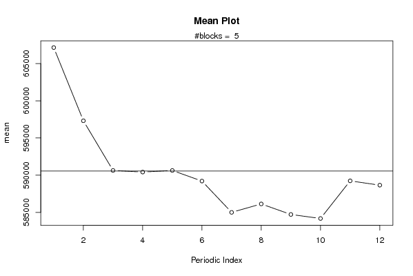
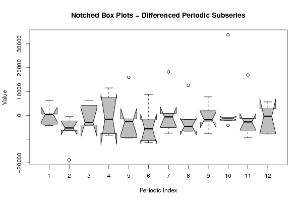
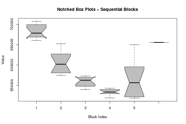
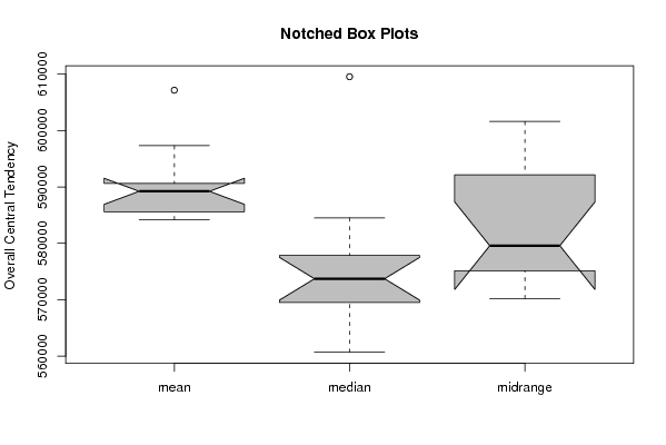
| Title produced by software | Mean Plot | ||||||||||||||||||||
| Date of computation | Sat, 12 Dec 2009 09:20:40 -0700 | ||||||||||||||||||||
| Cite this page as follows | Statistical Computations at FreeStatistics.org, Office for Research Development and Education, URL https://freestatistics.org/blog/index.php?v=date/2009/Dec/12/t12606349327tbh3ra4v87cwk4.htm/, Retrieved Mon, 29 Apr 2024 08:34:04 +0000 | ||||||||||||||||||||
| Statistical Computations at FreeStatistics.org, Office for Research Development and Education, URL https://freestatistics.org/blog/index.php?pk=67044, Retrieved Mon, 29 Apr 2024 08:34:04 +0000 | |||||||||||||||||||||
| QR Codes: | |||||||||||||||||||||
|
| |||||||||||||||||||||
| Original text written by user: | |||||||||||||||||||||
| IsPrivate? | No (this computation is public) | ||||||||||||||||||||
| User-defined keywords | |||||||||||||||||||||
| Estimated Impact | 126 | ||||||||||||||||||||
Tree of Dependent Computations | |||||||||||||||||||||
| Family? (F = Feedback message, R = changed R code, M = changed R Module, P = changed Parameters, D = changed Data) | |||||||||||||||||||||
| - [Bivariate Kernel Density Estimation] [Paper] [2009-12-12 13:34:31] [d31db4f83c6a129f6d3e47077769e868] - D [Bivariate Kernel Density Estimation] [Paper.1] [2009-12-12 13:38:38] [d31db4f83c6a129f6d3e47077769e868] - RMPD [Standard Deviation-Mean Plot] [Paper. Mean Plot ...] [2009-12-12 14:46:45] [d31db4f83c6a129f6d3e47077769e868] - D [Standard Deviation-Mean Plot] [Paper] [2009-12-12 14:54:21] [d31db4f83c6a129f6d3e47077769e868] - D [Standard Deviation-Mean Plot] [Paper. Ingeschrev...] [2009-12-12 15:28:35] [d31db4f83c6a129f6d3e47077769e868] - D [Standard Deviation-Mean Plot] [Paper. achtergest...] [2009-12-12 15:31:03] [d31db4f83c6a129f6d3e47077769e868] - RM D [Mean Plot] [Paper. Mean plot] [2009-12-12 16:13:07] [d31db4f83c6a129f6d3e47077769e868] - D [Mean Plot] [Paper. Inschrijvi...] [2009-12-12 16:18:27] [d31db4f83c6a129f6d3e47077769e868] - D [Mean Plot] [Paper. Mean plot ...] [2009-12-12 16:20:40] [852eae237d08746109043531619a60c9] [Current] | |||||||||||||||||||||
| Feedback Forum | |||||||||||||||||||||
Post a new message | |||||||||||||||||||||
Dataset | |||||||||||||||||||||
| Dataseries X: | |||||||||||||||||||||
707 169 703 434 701 017 696 968 688 558 679 237 677 362 676 693 670 009 667 209 662 976 660 194 652 270 648 024 629 295 624 961 617 306 607 691 596 219 591 130 584 528 576 798 575 683 574 369 566 815 573 074 567 739 571 942 570 274 568 800 558 115 550 591 548 872 547 009 545 946 539 702 542 427 542 968 536 640 533 653 540 996 538 316 532 646 533 390 528 715 530 664 528 564 519 107 518 703 519 059 518 498 524 575 536 046 552 006 560 687 578 884 591 491 599 228 633 019 649 918 655 509 | |||||||||||||||||||||
Tables (Output of Computation) | |||||||||||||||||||||
| |||||||||||||||||||||
Figures (Output of Computation) | |||||||||||||||||||||
Input Parameters & R Code | |||||||||||||||||||||
| Parameters (Session): | |||||||||||||||||||||
| par1 = 1 ; par2 = Do not include Seasonal Dummies ; par3 = No Linear Trend ; | |||||||||||||||||||||
| Parameters (R input): | |||||||||||||||||||||
| par1 = 12 ; | |||||||||||||||||||||
| R code (references can be found in the software module): | |||||||||||||||||||||
par1 <- as.numeric(par1) | |||||||||||||||||||||