Repository of Reproducible Computations

Free Statistics

of Irreproducible Research!

Author's title

Author

*Unverified author*

R Software Module

rwasp_autocorrelation.wasp

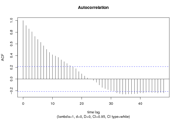
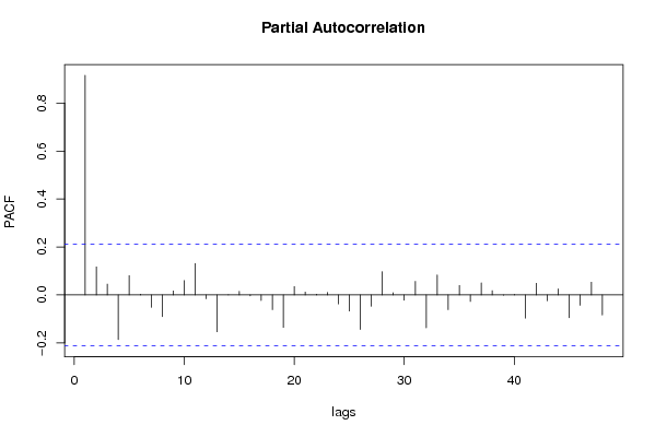
Title produced by software

(Partial) Autocorrelation Function

Date of computation

Sat, 12 Dec 2009 03:41:15 -0700

Cite this page as follows

Statistical Computations at FreeStatistics.org, Office for Research Development and Education, URL https://freestatistics.org/blog/index.php?v=date/2009/Dec/12/t1260614566qrsr4ytnjdomutz.htm/, Retrieved Mon, 29 Apr 2024 14:11:54 +0000

Statistical Computations at FreeStatistics.org, Office for Research Development and Education, URL https://freestatistics.org/blog/index.php?pk=66870, Retrieved Mon, 29 Apr 2024 14:11:54 +0000

QR Codes:

Paste this QR Code to cite your computation.

Original text written by user:

IsPrivate?

No (this computation is public)

User-defined keywords

KDGP2W21

Estimated Impact

147

Family? (F = Feedback message, R = changed R code, M = changed R Module, P = changed Parameters, D = changed Data)

-       [(Partial) Autocorrelation Function] [autocorrelatie ei...] [2009-12-12 10:41:15] [b37bab310ab56201887748d7a7c0dc58] [Current]

Feedback Forum

Post a new message

Dataseries X:

Download CSV

Histogram

Boxplots

1,2
1,21
1,21
1,21
1,21
1,21
1,21
1,2
1,21
1,22
1,22
1,23
1,22
1,23
1,23
1,23
1,23
1,23
1,22
1,22
1,23
1,24
1,24
1,25
1,25
1,25
1,26
1,26
1,26
1,26
1,27
1,27
1,29
1,31
1,32
1,32
1,33
1,33
1,32
1,32
1,31
1,3
1,31
1,29
1,3
1,3
1,32
1,31
1,35
1,35
1,36
1,37
1,37
1,37
1,32
1,32
1,31
1,31
1,34
1,31
1,27
1,28
1,27
1,26
1,27
1,27
1,28
1,27
1,26
1,3
1,31
1,28
1,29
1,31
1,29
1,29
1,32
1,3
1,29
1,31
1,29
1,33
1,35
1,32
1,33

Summary of computational transaction
Raw Input	view raw input (R code)
Raw Output	view raw output of R engine
Computing time	2 seconds
R Server	'Gwilym Jenkins' @ 72.249.127.135

\begin{tabular}{lllllllll}
\hline
Summary of computational transaction \tabularnewline
Raw Input & view raw input (R code)  \tabularnewline
Raw Output & view raw output of R engine  \tabularnewline
Computing time & 2 seconds \tabularnewline
R Server & 'Gwilym Jenkins' @ 72.249.127.135 \tabularnewline
\hline
\end{tabular}
%Source: https://freestatistics.org/blog/index.php?pk=66870&T=0

[TABLE]
[ROW][C]Summary of computational transaction[/C][/ROW]
[ROW][C]Raw Input[/C][C]view raw input (R code) [/C][/ROW]
[ROW][C]Raw Output[/C][C]view raw output of R engine [/C][/ROW]
[ROW][C]Computing time[/C][C]2 seconds[/C][/ROW]
[ROW][C]R Server[/C][C]'Gwilym Jenkins' @ 72.249.127.135[/C][/ROW]
[/TABLE]
Source: https://freestatistics.org/blog/index.php?pk=66870&T=0

Globally Unique Identifier (entire table): ba.freestatistics.org/blog/index.php?pk=66870&T=0

As an alternative you can also use a QR Code:

The GUIDs for individual cells are displayed in the table below:

Summary of computational transaction
Raw Input	view raw input (R code)
Raw Output	view raw output of R engine
Computing time	2 seconds
R Server	'Gwilym Jenkins' @ 72.249.127.135

Autocorrelation Function
Time lag k	ACF(k)	T-STAT	P-value
1	0.915696	8.4423	0
2	0.857424	7.9051	0
3	0.807622	7.4459	0
4	0.729536	6.726	0
5	0.678076	6.2516	0
6	0.6283	5.7926	0
7	0.568351	5.2399	1e-06
8	0.508402	4.6872	5e-06
9	0.456922	4.2126	3.1e-05
10	0.415076	3.8268	0.000124
11	0.394169	3.6341	0.000238
12	0.370979	3.4203	0.000482
13	0.328001	3.024	0.001649
14	0.29804	2.7478	0.003662
15	0.266361	2.4557	0.008048
16	0.231859	2.1376	0.017709
17	0.208702	1.9241	0.028842
18	0.178181	1.6428	0.052064
19	0.127287	1.1735	0.121931
20	0.089416	0.8244	0.206017
21	0.05267	0.4856	0.314252
22	0.018754	0.1729	0.431569
23	0.002375	0.0219	0.49129
24	-0.022506	-0.2075	0.418059
25	-0.057002	-0.5255	0.300292
26	-0.10171	-0.9377	0.175521
27	-0.144182	-1.3293	0.093654
28	-0.163997	-1.512	0.067125
29	-0.182679	-1.6842	0.047904
30	-0.201369	-1.8565	0.033421
31	-0.207048	-1.9089	0.029826
32	-0.23653	-2.1807	0.015984
33	-0.247915	-2.2857	0.012381
34	-0.258182	-2.3803	0.009767
35	-0.259394	-2.3915	0.009493
36	-0.256072	-2.3609	0.01026
37	-0.25502	-2.3512	0.010514
38	-0.252243	-2.3256	0.011212
39	-0.250033	-2.3052	0.011796
40	-0.238188	-2.196	0.015408
41	-0.239354	-2.2067	0.015014
42	-0.229753	-2.1182	0.018538
43	-0.226397	-2.0873	0.019929
44	-0.232077	-2.1396	0.017625
45	-0.233808	-2.1556	0.016971
46	-0.238375	-2.1977	0.015345
47	-0.231637	-2.1356	0.017795
48	-0.237916	-2.1935	0.015502

\begin{tabular}{lllllllll}
\hline
Autocorrelation Function \tabularnewline
Time lag k & ACF(k) & T-STAT & P-value \tabularnewline
1 & 0.915696 & 8.4423 & 0 \tabularnewline
2 & 0.857424 & 7.9051 & 0 \tabularnewline
3 & 0.807622 & 7.4459 & 0 \tabularnewline
4 & 0.729536 & 6.726 & 0 \tabularnewline
5 & 0.678076 & 6.2516 & 0 \tabularnewline
6 & 0.6283 & 5.7926 & 0 \tabularnewline
7 & 0.568351 & 5.2399 & 1e-06 \tabularnewline
8 & 0.508402 & 4.6872 & 5e-06 \tabularnewline
9 & 0.456922 & 4.2126 & 3.1e-05 \tabularnewline
10 & 0.415076 & 3.8268 & 0.000124 \tabularnewline
11 & 0.394169 & 3.6341 & 0.000238 \tabularnewline
12 & 0.370979 & 3.4203 & 0.000482 \tabularnewline
13 & 0.328001 & 3.024 & 0.001649 \tabularnewline
14 & 0.29804 & 2.7478 & 0.003662 \tabularnewline
15 & 0.266361 & 2.4557 & 0.008048 \tabularnewline
16 & 0.231859 & 2.1376 & 0.017709 \tabularnewline
17 & 0.208702 & 1.9241 & 0.028842 \tabularnewline
18 & 0.178181 & 1.6428 & 0.052064 \tabularnewline
19 & 0.127287 & 1.1735 & 0.121931 \tabularnewline
20 & 0.089416 & 0.8244 & 0.206017 \tabularnewline
21 & 0.05267 & 0.4856 & 0.314252 \tabularnewline
22 & 0.018754 & 0.1729 & 0.431569 \tabularnewline
23 & 0.002375 & 0.0219 & 0.49129 \tabularnewline
24 & -0.022506 & -0.2075 & 0.418059 \tabularnewline
25 & -0.057002 & -0.5255 & 0.300292 \tabularnewline
26 & -0.10171 & -0.9377 & 0.175521 \tabularnewline
27 & -0.144182 & -1.3293 & 0.093654 \tabularnewline
28 & -0.163997 & -1.512 & 0.067125 \tabularnewline
29 & -0.182679 & -1.6842 & 0.047904 \tabularnewline
30 & -0.201369 & -1.8565 & 0.033421 \tabularnewline
31 & -0.207048 & -1.9089 & 0.029826 \tabularnewline
32 & -0.23653 & -2.1807 & 0.015984 \tabularnewline
33 & -0.247915 & -2.2857 & 0.012381 \tabularnewline
34 & -0.258182 & -2.3803 & 0.009767 \tabularnewline
35 & -0.259394 & -2.3915 & 0.009493 \tabularnewline
36 & -0.256072 & -2.3609 & 0.01026 \tabularnewline
37 & -0.25502 & -2.3512 & 0.010514 \tabularnewline
38 & -0.252243 & -2.3256 & 0.011212 \tabularnewline
39 & -0.250033 & -2.3052 & 0.011796 \tabularnewline
40 & -0.238188 & -2.196 & 0.015408 \tabularnewline
41 & -0.239354 & -2.2067 & 0.015014 \tabularnewline
42 & -0.229753 & -2.1182 & 0.018538 \tabularnewline
43 & -0.226397 & -2.0873 & 0.019929 \tabularnewline
44 & -0.232077 & -2.1396 & 0.017625 \tabularnewline
45 & -0.233808 & -2.1556 & 0.016971 \tabularnewline
46 & -0.238375 & -2.1977 & 0.015345 \tabularnewline
47 & -0.231637 & -2.1356 & 0.017795 \tabularnewline
48 & -0.237916 & -2.1935 & 0.015502 \tabularnewline
\hline
\end{tabular}
%Source: https://freestatistics.org/blog/index.php?pk=66870&T=1

[TABLE]
[ROW][C]Autocorrelation Function[/C][/ROW]
[ROW][C]Time lag k[/C][C]ACF(k)[/C][C]T-STAT[/C][C]P-value[/C][/ROW]
[ROW][C]1[/C][C]0.915696[/C][C]8.4423[/C][C]0[/C][/ROW]
[ROW][C]2[/C][C]0.857424[/C][C]7.9051[/C][C]0[/C][/ROW]
[ROW][C]3[/C][C]0.807622[/C][C]7.4459[/C][C]0[/C][/ROW]
[ROW][C]4[/C][C]0.729536[/C][C]6.726[/C][C]0[/C][/ROW]
[ROW][C]5[/C][C]0.678076[/C][C]6.2516[/C][C]0[/C][/ROW]
[ROW][C]6[/C][C]0.6283[/C][C]5.7926[/C][C]0[/C][/ROW]
[ROW][C]7[/C][C]0.568351[/C][C]5.2399[/C][C]1e-06[/C][/ROW]
[ROW][C]8[/C][C]0.508402[/C][C]4.6872[/C][C]5e-06[/C][/ROW]
[ROW][C]9[/C][C]0.456922[/C][C]4.2126[/C][C]3.1e-05[/C][/ROW]
[ROW][C]10[/C][C]0.415076[/C][C]3.8268[/C][C]0.000124[/C][/ROW]
[ROW][C]11[/C][C]0.394169[/C][C]3.6341[/C][C]0.000238[/C][/ROW]
[ROW][C]12[/C][C]0.370979[/C][C]3.4203[/C][C]0.000482[/C][/ROW]
[ROW][C]13[/C][C]0.328001[/C][C]3.024[/C][C]0.001649[/C][/ROW]
[ROW][C]14[/C][C]0.29804[/C][C]2.7478[/C][C]0.003662[/C][/ROW]
[ROW][C]15[/C][C]0.266361[/C][C]2.4557[/C][C]0.008048[/C][/ROW]
[ROW][C]16[/C][C]0.231859[/C][C]2.1376[/C][C]0.017709[/C][/ROW]
[ROW][C]17[/C][C]0.208702[/C][C]1.9241[/C][C]0.028842[/C][/ROW]
[ROW][C]18[/C][C]0.178181[/C][C]1.6428[/C][C]0.052064[/C][/ROW]
[ROW][C]19[/C][C]0.127287[/C][C]1.1735[/C][C]0.121931[/C][/ROW]
[ROW][C]20[/C][C]0.089416[/C][C]0.8244[/C][C]0.206017[/C][/ROW]
[ROW][C]21[/C][C]0.05267[/C][C]0.4856[/C][C]0.314252[/C][/ROW]
[ROW][C]22[/C][C]0.018754[/C][C]0.1729[/C][C]0.431569[/C][/ROW]
[ROW][C]23[/C][C]0.002375[/C][C]0.0219[/C][C]0.49129[/C][/ROW]
[ROW][C]24[/C][C]-0.022506[/C][C]-0.2075[/C][C]0.418059[/C][/ROW]
[ROW][C]25[/C][C]-0.057002[/C][C]-0.5255[/C][C]0.300292[/C][/ROW]
[ROW][C]26[/C][C]-0.10171[/C][C]-0.9377[/C][C]0.175521[/C][/ROW]
[ROW][C]27[/C][C]-0.144182[/C][C]-1.3293[/C][C]0.093654[/C][/ROW]
[ROW][C]28[/C][C]-0.163997[/C][C]-1.512[/C][C]0.067125[/C][/ROW]
[ROW][C]29[/C][C]-0.182679[/C][C]-1.6842[/C][C]0.047904[/C][/ROW]
[ROW][C]30[/C][C]-0.201369[/C][C]-1.8565[/C][C]0.033421[/C][/ROW]
[ROW][C]31[/C][C]-0.207048[/C][C]-1.9089[/C][C]0.029826[/C][/ROW]
[ROW][C]32[/C][C]-0.23653[/C][C]-2.1807[/C][C]0.015984[/C][/ROW]
[ROW][C]33[/C][C]-0.247915[/C][C]-2.2857[/C][C]0.012381[/C][/ROW]
[ROW][C]34[/C][C]-0.258182[/C][C]-2.3803[/C][C]0.009767[/C][/ROW]
[ROW][C]35[/C][C]-0.259394[/C][C]-2.3915[/C][C]0.009493[/C][/ROW]
[ROW][C]36[/C][C]-0.256072[/C][C]-2.3609[/C][C]0.01026[/C][/ROW]
[ROW][C]37[/C][C]-0.25502[/C][C]-2.3512[/C][C]0.010514[/C][/ROW]
[ROW][C]38[/C][C]-0.252243[/C][C]-2.3256[/C][C]0.011212[/C][/ROW]
[ROW][C]39[/C][C]-0.250033[/C][C]-2.3052[/C][C]0.011796[/C][/ROW]
[ROW][C]40[/C][C]-0.238188[/C][C]-2.196[/C][C]0.015408[/C][/ROW]
[ROW][C]41[/C][C]-0.239354[/C][C]-2.2067[/C][C]0.015014[/C][/ROW]
[ROW][C]42[/C][C]-0.229753[/C][C]-2.1182[/C][C]0.018538[/C][/ROW]
[ROW][C]43[/C][C]-0.226397[/C][C]-2.0873[/C][C]0.019929[/C][/ROW]
[ROW][C]44[/C][C]-0.232077[/C][C]-2.1396[/C][C]0.017625[/C][/ROW]
[ROW][C]45[/C][C]-0.233808[/C][C]-2.1556[/C][C]0.016971[/C][/ROW]
[ROW][C]46[/C][C]-0.238375[/C][C]-2.1977[/C][C]0.015345[/C][/ROW]
[ROW][C]47[/C][C]-0.231637[/C][C]-2.1356[/C][C]0.017795[/C][/ROW]
[ROW][C]48[/C][C]-0.237916[/C][C]-2.1935[/C][C]0.015502[/C][/ROW]
[/TABLE]
Source: https://freestatistics.org/blog/index.php?pk=66870&T=1

Globally Unique Identifier (entire table): ba.freestatistics.org/blog/index.php?pk=66870&T=1

As an alternative you can also use a QR Code:

The GUIDs for individual cells are displayed in the table below:

Autocorrelation Function
Time lag k	ACF(k)	T-STAT	P-value
1	0.915696	8.4423	0
2	0.857424	7.9051	0
3	0.807622	7.4459	0
4	0.729536	6.726	0
5	0.678076	6.2516	0
6	0.6283	5.7926	0
7	0.568351	5.2399	1e-06
8	0.508402	4.6872	5e-06
9	0.456922	4.2126	3.1e-05
10	0.415076	3.8268	0.000124
11	0.394169	3.6341	0.000238
12	0.370979	3.4203	0.000482
13	0.328001	3.024	0.001649
14	0.29804	2.7478	0.003662
15	0.266361	2.4557	0.008048
16	0.231859	2.1376	0.017709
17	0.208702	1.9241	0.028842
18	0.178181	1.6428	0.052064
19	0.127287	1.1735	0.121931
20	0.089416	0.8244	0.206017
21	0.05267	0.4856	0.314252
22	0.018754	0.1729	0.431569
23	0.002375	0.0219	0.49129
24	-0.022506	-0.2075	0.418059
25	-0.057002	-0.5255	0.300292
26	-0.10171	-0.9377	0.175521
27	-0.144182	-1.3293	0.093654
28	-0.163997	-1.512	0.067125
29	-0.182679	-1.6842	0.047904
30	-0.201369	-1.8565	0.033421
31	-0.207048	-1.9089	0.029826
32	-0.23653	-2.1807	0.015984
33	-0.247915	-2.2857	0.012381
34	-0.258182	-2.3803	0.009767
35	-0.259394	-2.3915	0.009493
36	-0.256072	-2.3609	0.01026
37	-0.25502	-2.3512	0.010514
38	-0.252243	-2.3256	0.011212
39	-0.250033	-2.3052	0.011796
40	-0.238188	-2.196	0.015408
41	-0.239354	-2.2067	0.015014
42	-0.229753	-2.1182	0.018538
43	-0.226397	-2.0873	0.019929
44	-0.232077	-2.1396	0.017625
45	-0.233808	-2.1556	0.016971
46	-0.238375	-2.1977	0.015345
47	-0.231637	-2.1356	0.017795
48	-0.237916	-2.1935	0.015502

Partial Autocorrelation Function
Time lag k	PACF(k)	T-STAT	P-value
1	0.915696	8.4423	0
2	0.117186	1.0804	0.141509
3	0.045095	0.4158	0.339318
4	-0.186105	-1.7158	0.04492
5	0.080302	0.7403	0.230565
6	0.002917	0.0269	0.489303
7	-0.051517	-0.475	0.318017
8	-0.090485	-0.8342	0.203246
9	0.016881	0.1556	0.438344
10	0.05979	0.5512	0.291459
11	0.131318	1.2107	0.114685
12	-0.015895	-0.1465	0.441919
13	-0.153265	-1.413	0.080649
14	8e-04	0.0074	0.497067
15	0.015256	0.1407	0.444237
16	-0.003615	-0.0333	0.486745
17	-0.023329	-0.2151	0.415109
18	-0.061318	-0.5653	0.286672
19	-0.135513	-1.2494	0.107479
20	0.034702	0.3199	0.374901
21	0.012163	0.1121	0.455488
22	0.003044	0.0281	0.488839
23	0.010431	0.0962	0.461807
24	-0.037571	-0.3464	0.364955
25	-0.067247	-0.62	0.268463
26	-0.143698	-1.3248	0.094389
27	-0.047233	-0.4355	0.332163
28	0.097246	0.8966	0.186243
29	0.009094	0.0838	0.46669
30	-0.022173	-0.2044	0.419256
31	0.056619	0.522	0.301513
32	-0.137062	-1.2637	0.104905
33	0.083515	0.77	0.221726
34	-0.061073	-0.5631	0.287436
35	0.039511	0.3643	0.358279
36	-0.027323	-0.2519	0.40086
37	0.050532	0.4659	0.321247
38	0.017721	0.1634	0.435303
39	-0.000672	-0.0062	0.497535
40	0.00251	0.0231	0.490796
41	-0.096893	-0.8933	0.187107
42	0.048713	0.4491	0.327248
43	-0.024197	-0.2231	0.412003
44	0.02505	0.2309	0.408955
45	-0.094834	-0.8743	0.192201
46	-0.042944	-0.3959	0.346578
47	0.053152	0.49	0.312684
48	-0.083712	-0.7718	0.22119

\begin{tabular}{lllllllll}
\hline
Partial Autocorrelation Function \tabularnewline
Time lag k & PACF(k) & T-STAT & P-value \tabularnewline
1 & 0.915696 & 8.4423 & 0 \tabularnewline
2 & 0.117186 & 1.0804 & 0.141509 \tabularnewline
3 & 0.045095 & 0.4158 & 0.339318 \tabularnewline
4 & -0.186105 & -1.7158 & 0.04492 \tabularnewline
5 & 0.080302 & 0.7403 & 0.230565 \tabularnewline
6 & 0.002917 & 0.0269 & 0.489303 \tabularnewline
7 & -0.051517 & -0.475 & 0.318017 \tabularnewline
8 & -0.090485 & -0.8342 & 0.203246 \tabularnewline
9 & 0.016881 & 0.1556 & 0.438344 \tabularnewline
10 & 0.05979 & 0.5512 & 0.291459 \tabularnewline
11 & 0.131318 & 1.2107 & 0.114685 \tabularnewline
12 & -0.015895 & -0.1465 & 0.441919 \tabularnewline
13 & -0.153265 & -1.413 & 0.080649 \tabularnewline
14 & 8e-04 & 0.0074 & 0.497067 \tabularnewline
15 & 0.015256 & 0.1407 & 0.444237 \tabularnewline
16 & -0.003615 & -0.0333 & 0.486745 \tabularnewline
17 & -0.023329 & -0.2151 & 0.415109 \tabularnewline
18 & -0.061318 & -0.5653 & 0.286672 \tabularnewline
19 & -0.135513 & -1.2494 & 0.107479 \tabularnewline
20 & 0.034702 & 0.3199 & 0.374901 \tabularnewline
21 & 0.012163 & 0.1121 & 0.455488 \tabularnewline
22 & 0.003044 & 0.0281 & 0.488839 \tabularnewline
23 & 0.010431 & 0.0962 & 0.461807 \tabularnewline
24 & -0.037571 & -0.3464 & 0.364955 \tabularnewline
25 & -0.067247 & -0.62 & 0.268463 \tabularnewline
26 & -0.143698 & -1.3248 & 0.094389 \tabularnewline
27 & -0.047233 & -0.4355 & 0.332163 \tabularnewline
28 & 0.097246 & 0.8966 & 0.186243 \tabularnewline
29 & 0.009094 & 0.0838 & 0.46669 \tabularnewline
30 & -0.022173 & -0.2044 & 0.419256 \tabularnewline
31 & 0.056619 & 0.522 & 0.301513 \tabularnewline
32 & -0.137062 & -1.2637 & 0.104905 \tabularnewline
33 & 0.083515 & 0.77 & 0.221726 \tabularnewline
34 & -0.061073 & -0.5631 & 0.287436 \tabularnewline
35 & 0.039511 & 0.3643 & 0.358279 \tabularnewline
36 & -0.027323 & -0.2519 & 0.40086 \tabularnewline
37 & 0.050532 & 0.4659 & 0.321247 \tabularnewline
38 & 0.017721 & 0.1634 & 0.435303 \tabularnewline
39 & -0.000672 & -0.0062 & 0.497535 \tabularnewline
40 & 0.00251 & 0.0231 & 0.490796 \tabularnewline
41 & -0.096893 & -0.8933 & 0.187107 \tabularnewline
42 & 0.048713 & 0.4491 & 0.327248 \tabularnewline
43 & -0.024197 & -0.2231 & 0.412003 \tabularnewline
44 & 0.02505 & 0.2309 & 0.408955 \tabularnewline
45 & -0.094834 & -0.8743 & 0.192201 \tabularnewline
46 & -0.042944 & -0.3959 & 0.346578 \tabularnewline
47 & 0.053152 & 0.49 & 0.312684 \tabularnewline
48 & -0.083712 & -0.7718 & 0.22119 \tabularnewline
\hline
\end{tabular}
%Source: https://freestatistics.org/blog/index.php?pk=66870&T=2

[TABLE]
[ROW][C]Partial Autocorrelation Function[/C][/ROW]
[ROW][C]Time lag k[/C][C]PACF(k)[/C][C]T-STAT[/C][C]P-value[/C][/ROW]
[ROW][C]1[/C][C]0.915696[/C][C]8.4423[/C][C]0[/C][/ROW]
[ROW][C]2[/C][C]0.117186[/C][C]1.0804[/C][C]0.141509[/C][/ROW]
[ROW][C]3[/C][C]0.045095[/C][C]0.4158[/C][C]0.339318[/C][/ROW]
[ROW][C]4[/C][C]-0.186105[/C][C]-1.7158[/C][C]0.04492[/C][/ROW]
[ROW][C]5[/C][C]0.080302[/C][C]0.7403[/C][C]0.230565[/C][/ROW]
[ROW][C]6[/C][C]0.002917[/C][C]0.0269[/C][C]0.489303[/C][/ROW]
[ROW][C]7[/C][C]-0.051517[/C][C]-0.475[/C][C]0.318017[/C][/ROW]
[ROW][C]8[/C][C]-0.090485[/C][C]-0.8342[/C][C]0.203246[/C][/ROW]
[ROW][C]9[/C][C]0.016881[/C][C]0.1556[/C][C]0.438344[/C][/ROW]
[ROW][C]10[/C][C]0.05979[/C][C]0.5512[/C][C]0.291459[/C][/ROW]
[ROW][C]11[/C][C]0.131318[/C][C]1.2107[/C][C]0.114685[/C][/ROW]
[ROW][C]12[/C][C]-0.015895[/C][C]-0.1465[/C][C]0.441919[/C][/ROW]
[ROW][C]13[/C][C]-0.153265[/C][C]-1.413[/C][C]0.080649[/C][/ROW]
[ROW][C]14[/C][C]8e-04[/C][C]0.0074[/C][C]0.497067[/C][/ROW]
[ROW][C]15[/C][C]0.015256[/C][C]0.1407[/C][C]0.444237[/C][/ROW]
[ROW][C]16[/C][C]-0.003615[/C][C]-0.0333[/C][C]0.486745[/C][/ROW]
[ROW][C]17[/C][C]-0.023329[/C][C]-0.2151[/C][C]0.415109[/C][/ROW]
[ROW][C]18[/C][C]-0.061318[/C][C]-0.5653[/C][C]0.286672[/C][/ROW]
[ROW][C]19[/C][C]-0.135513[/C][C]-1.2494[/C][C]0.107479[/C][/ROW]
[ROW][C]20[/C][C]0.034702[/C][C]0.3199[/C][C]0.374901[/C][/ROW]
[ROW][C]21[/C][C]0.012163[/C][C]0.1121[/C][C]0.455488[/C][/ROW]
[ROW][C]22[/C][C]0.003044[/C][C]0.0281[/C][C]0.488839[/C][/ROW]
[ROW][C]23[/C][C]0.010431[/C][C]0.0962[/C][C]0.461807[/C][/ROW]
[ROW][C]24[/C][C]-0.037571[/C][C]-0.3464[/C][C]0.364955[/C][/ROW]
[ROW][C]25[/C][C]-0.067247[/C][C]-0.62[/C][C]0.268463[/C][/ROW]
[ROW][C]26[/C][C]-0.143698[/C][C]-1.3248[/C][C]0.094389[/C][/ROW]
[ROW][C]27[/C][C]-0.047233[/C][C]-0.4355[/C][C]0.332163[/C][/ROW]
[ROW][C]28[/C][C]0.097246[/C][C]0.8966[/C][C]0.186243[/C][/ROW]
[ROW][C]29[/C][C]0.009094[/C][C]0.0838[/C][C]0.46669[/C][/ROW]
[ROW][C]30[/C][C]-0.022173[/C][C]-0.2044[/C][C]0.419256[/C][/ROW]
[ROW][C]31[/C][C]0.056619[/C][C]0.522[/C][C]0.301513[/C][/ROW]
[ROW][C]32[/C][C]-0.137062[/C][C]-1.2637[/C][C]0.104905[/C][/ROW]
[ROW][C]33[/C][C]0.083515[/C][C]0.77[/C][C]0.221726[/C][/ROW]
[ROW][C]34[/C][C]-0.061073[/C][C]-0.5631[/C][C]0.287436[/C][/ROW]
[ROW][C]35[/C][C]0.039511[/C][C]0.3643[/C][C]0.358279[/C][/ROW]
[ROW][C]36[/C][C]-0.027323[/C][C]-0.2519[/C][C]0.40086[/C][/ROW]
[ROW][C]37[/C][C]0.050532[/C][C]0.4659[/C][C]0.321247[/C][/ROW]
[ROW][C]38[/C][C]0.017721[/C][C]0.1634[/C][C]0.435303[/C][/ROW]
[ROW][C]39[/C][C]-0.000672[/C][C]-0.0062[/C][C]0.497535[/C][/ROW]
[ROW][C]40[/C][C]0.00251[/C][C]0.0231[/C][C]0.490796[/C][/ROW]
[ROW][C]41[/C][C]-0.096893[/C][C]-0.8933[/C][C]0.187107[/C][/ROW]
[ROW][C]42[/C][C]0.048713[/C][C]0.4491[/C][C]0.327248[/C][/ROW]
[ROW][C]43[/C][C]-0.024197[/C][C]-0.2231[/C][C]0.412003[/C][/ROW]
[ROW][C]44[/C][C]0.02505[/C][C]0.2309[/C][C]0.408955[/C][/ROW]
[ROW][C]45[/C][C]-0.094834[/C][C]-0.8743[/C][C]0.192201[/C][/ROW]
[ROW][C]46[/C][C]-0.042944[/C][C]-0.3959[/C][C]0.346578[/C][/ROW]
[ROW][C]47[/C][C]0.053152[/C][C]0.49[/C][C]0.312684[/C][/ROW]
[ROW][C]48[/C][C]-0.083712[/C][C]-0.7718[/C][C]0.22119[/C][/ROW]
[/TABLE]
Source: https://freestatistics.org/blog/index.php?pk=66870&T=2

Globally Unique Identifier (entire table): ba.freestatistics.org/blog/index.php?pk=66870&T=2

As an alternative you can also use a QR Code:

The GUIDs for individual cells are displayed in the table below:

Partial Autocorrelation Function
Time lag k	PACF(k)	T-STAT	P-value
1	0.915696	8.4423	0
2	0.117186	1.0804	0.141509
3	0.045095	0.4158	0.339318
4	-0.186105	-1.7158	0.04492
5	0.080302	0.7403	0.230565
6	0.002917	0.0269	0.489303
7	-0.051517	-0.475	0.318017
8	-0.090485	-0.8342	0.203246
9	0.016881	0.1556	0.438344
10	0.05979	0.5512	0.291459
11	0.131318	1.2107	0.114685
12	-0.015895	-0.1465	0.441919
13	-0.153265	-1.413	0.080649
14	8e-04	0.0074	0.497067
15	0.015256	0.1407	0.444237
16	-0.003615	-0.0333	0.486745
17	-0.023329	-0.2151	0.415109
18	-0.061318	-0.5653	0.286672
19	-0.135513	-1.2494	0.107479
20	0.034702	0.3199	0.374901
21	0.012163	0.1121	0.455488
22	0.003044	0.0281	0.488839
23	0.010431	0.0962	0.461807
24	-0.037571	-0.3464	0.364955
25	-0.067247	-0.62	0.268463
26	-0.143698	-1.3248	0.094389
27	-0.047233	-0.4355	0.332163
28	0.097246	0.8966	0.186243
29	0.009094	0.0838	0.46669
30	-0.022173	-0.2044	0.419256
31	0.056619	0.522	0.301513
32	-0.137062	-1.2637	0.104905
33	0.083515	0.77	0.221726
34	-0.061073	-0.5631	0.287436
35	0.039511	0.3643	0.358279
36	-0.027323	-0.2519	0.40086
37	0.050532	0.4659	0.321247
38	0.017721	0.1634	0.435303
39	-0.000672	-0.0062	0.497535
40	0.00251	0.0231	0.490796
41	-0.096893	-0.8933	0.187107
42	0.048713	0.4491	0.327248
43	-0.024197	-0.2231	0.412003
44	0.02505	0.2309	0.408955
45	-0.094834	-0.8743	0.192201
46	-0.042944	-0.3959	0.346578
47	0.053152	0.49	0.312684
48	-0.083712	-0.7718	0.22119

Figure 1

PNG link

Postscript link

PDF link

Figure 2

PNG link

Postscript link

PDF link

Parameters (Session):

par1 = 48 ; par2 = 1 ; par3 = 0 ; par4 = 0 ; par5 = 12 ; par6 = White Noise ; par7 = 0.95 ;

Parameters (R input):

par1 = 48 ; par2 = 1 ; par3 = 0 ; par4 = 0 ; par5 = 12 ; par6 = White Noise ; par7 = 0.95 ;

R code (references can be found in the software module):

if (par1 == 'Default') {
par1 = 10*log10(length(x))
} else {
par1 <- as.numeric(par1)
}
par2 <- as.numeric(par2)
par3 <- as.numeric(par3)
par4 <- as.numeric(par4)
par5 <- as.numeric(par5)
if (par6 == 'White Noise') par6 <- 'white' else par6 <- 'ma'
par7 <- as.numeric(par7)
if (par2 == 0) {
x <- log(x)
} else {
x <- (x ^ par2 - 1) / par2
}
if (par3 > 0) x <- diff(x,lag=1,difference=par3)
if (par4 > 0) x <- diff(x,lag=par5,difference=par4)
bitmap(file='pic1.png')
racf <- acf(x, par1, main='Autocorrelation', xlab='time lag', ylab='ACF', ci.type=par6, ci=par7, sub=paste('(lambda=',par2,', d=',par3,', D=',par4,', CI=', par7, ', CI type=',par6,')',sep=''))
dev.off()
bitmap(file='pic2.png')
rpacf <- pacf(x,par1,main='Partial Autocorrelation',xlab='lags',ylab='PACF')
dev.off()
(myacf <- c(racf$acf))
(mypacf <- c(rpacf$acf))
lengthx <- length(x)
sqrtn <- sqrt(lengthx)
load(file='createtable')
a<-table.start()
a<-table.row.start(a)
a<-table.element(a,'Autocorrelation Function',4,TRUE)
a<-table.row.end(a)
a<-table.row.start(a)
a<-table.element(a,'Time lag k',header=TRUE)
a<-table.element(a,hyperlink('basics.htm','ACF(k)','click here for more information about the Autocorrelation Function'),header=TRUE)
a<-table.element(a,'T-STAT',header=TRUE)
a<-table.element(a,'P-value',header=TRUE)
a<-table.row.end(a)
for (i in 2:(par1+1)) {
a<-table.row.start(a)
a<-table.element(a,i-1,header=TRUE)
a<-table.element(a,round(myacf[i],6))
mytstat <- myacf[i]*sqrtn
a<-table.element(a,round(mytstat,4))
a<-table.element(a,round(1-pt(abs(mytstat),lengthx),6))
a<-table.row.end(a)
}
a<-table.end(a)
table.save(a,file='mytable.tab')
a<-table.start()
a<-table.row.start(a)
a<-table.element(a,'Partial Autocorrelation Function',4,TRUE)
a<-table.row.end(a)
a<-table.row.start(a)
a<-table.element(a,'Time lag k',header=TRUE)
a<-table.element(a,hyperlink('basics.htm','PACF(k)','click here for more information about the Partial Autocorrelation Function'),header=TRUE)
a<-table.element(a,'T-STAT',header=TRUE)
a<-table.element(a,'P-value',header=TRUE)
a<-table.row.end(a)
for (i in 1:par1) {
a<-table.row.start(a)
a<-table.element(a,i,header=TRUE)
a<-table.element(a,round(mypacf[i],6))
mytstat <- mypacf[i]*sqrtn
a<-table.element(a,round(mytstat,4))
a<-table.element(a,round(1-pt(abs(mytstat),lengthx),6))
a<-table.row.end(a)
}
a<-table.end(a)
table.save(a,file='mytable1.tab')

Free Statistics

Description of Statistical Computation

Tree of Dependent Computations

Dataset

Tables (Output of Computation)

Figures (Output of Computation)

Input Parameters & R Code