Free Statistics
of Irreproducible Research!
Description of Statistical Computation | |||||||||||||||||||||||||||||||||||||||||||||||||||||
|---|---|---|---|---|---|---|---|---|---|---|---|---|---|---|---|---|---|---|---|---|---|---|---|---|---|---|---|---|---|---|---|---|---|---|---|---|---|---|---|---|---|---|---|---|---|---|---|---|---|---|---|---|---|
| Author's title | |||||||||||||||||||||||||||||||||||||||||||||||||||||
| Author | *The author of this computation has been verified* | ||||||||||||||||||||||||||||||||||||||||||||||||||||
| R Software Module | rwasp_edauni.wasp | ||||||||||||||||||||||||||||||||||||||||||||||||||||
| Title produced by software | Univariate Explorative Data Analysis | ||||||||||||||||||||||||||||||||||||||||||||||||||||
| Date of computation | Fri, 11 Dec 2009 13:05:01 -0700 | ||||||||||||||||||||||||||||||||||||||||||||||||||||
| Cite this page as follows | Statistical Computations at FreeStatistics.org, Office for Research Development and Education, URL https://freestatistics.org/blog/index.php?v=date/2009/Dec/11/t1260561938ztqhpqftdmhyrh9.htm/, Retrieved Mon, 29 Apr 2024 00:50:08 +0000 | ||||||||||||||||||||||||||||||||||||||||||||||||||||
| Statistical Computations at FreeStatistics.org, Office for Research Development and Education, URL https://freestatistics.org/blog/index.php?pk=66740, Retrieved Mon, 29 Apr 2024 00:50:08 +0000 | |||||||||||||||||||||||||||||||||||||||||||||||||||||
| QR Codes: | |||||||||||||||||||||||||||||||||||||||||||||||||||||
|
| |||||||||||||||||||||||||||||||||||||||||||||||||||||
| Original text written by user: | |||||||||||||||||||||||||||||||||||||||||||||||||||||
| IsPrivate? | No (this computation is public) | ||||||||||||||||||||||||||||||||||||||||||||||||||||
| User-defined keywords | |||||||||||||||||||||||||||||||||||||||||||||||||||||
| Estimated Impact | 161 | ||||||||||||||||||||||||||||||||||||||||||||||||||||
Tree of Dependent Computations | |||||||||||||||||||||||||||||||||||||||||||||||||||||
| Family? (F = Feedback message, R = changed R code, M = changed R Module, P = changed Parameters, D = changed Data) | |||||||||||||||||||||||||||||||||||||||||||||||||||||
| - [Univariate Data Series] [data set] [2008-12-01 19:54:57] [b98453cac15ba1066b407e146608df68] - RMP [ARIMA Backward Selection] [] [2009-11-27 14:53:14] [b98453cac15ba1066b407e146608df68] - PD [ARIMA Backward Selection] [WS9] [2009-12-03 23:50:09] [37a8d600db9abe09a2528d150ccff095] - RMPD [Harrell-Davis Quantiles] [] [2009-12-04 21:24:16] [74be16979710d4c4e7c6647856088456] - RMP [Univariate Explorative Data Analysis] [] [2009-12-04 21:35:31] [74be16979710d4c4e7c6647856088456] - D [Univariate Explorative Data Analysis] [] [2009-12-11 20:05:01] [d41d8cd98f00b204e9800998ecf8427e] [Current] - D [Univariate Explorative Data Analysis] [] [2009-12-14 17:14:02] [74be16979710d4c4e7c6647856088456] | |||||||||||||||||||||||||||||||||||||||||||||||||||||
| Feedback Forum | |||||||||||||||||||||||||||||||||||||||||||||||||||||
Post a new message | |||||||||||||||||||||||||||||||||||||||||||||||||||||
Dataset | |||||||||||||||||||||||||||||||||||||||||||||||||||||
| Dataseries X: | |||||||||||||||||||||||||||||||||||||||||||||||||||||
-0.0175986496695149 4.88533001639715e-06 -0.0797142045361252 0.0380359724366437 0.00379990057404902 0.0592823368877745 -0.0401047028912839 -0.0903371585255128 0.0600435985327014 -0.0751519168673696 0.184740243449584 0.108923749072312 0.148749967789766 0.0299253269806808 -0.132723413231867 0.130073522884216 -0.0524172791064149 -0.0488662775462986 0.0210676927748520 -0.165146636794414 -0.0573375413155754 0.00334278216483919 -0.120892947016097 0.0140181973103131 -0.166333957140904 -0.204256136740815 -0.170162160910135 -0.40685370432818 0.089890889862059 0.121852449126500 0.0718684968241188 0.146330323762528 -0.254402885578116 -0.175254145082071 0.0883657966655966 0.0494861859369645 -0.179560126045166 0.0352805435009704 0.107242027471589 0.0159604480893762 0.229492599513338 -0.472622684816943 -0.0310496393734398 0.0823390463619987 -0.0459447059808648 -0.0671207054879601 0.062392997118939 0.0541581853860086 -0.000768654964170624 | |||||||||||||||||||||||||||||||||||||||||||||||||||||
Tables (Output of Computation) | |||||||||||||||||||||||||||||||||||||||||||||||||||||
| |||||||||||||||||||||||||||||||||||||||||||||||||||||
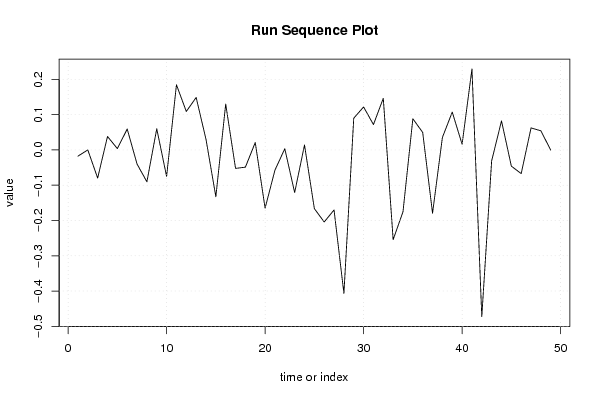
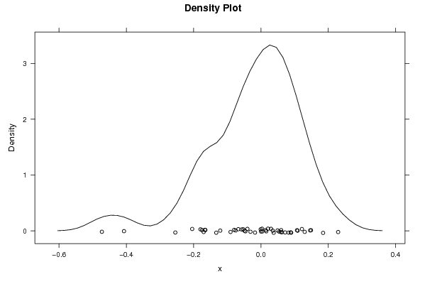
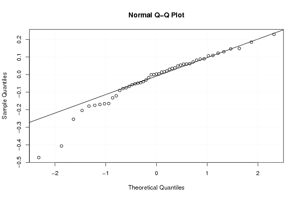
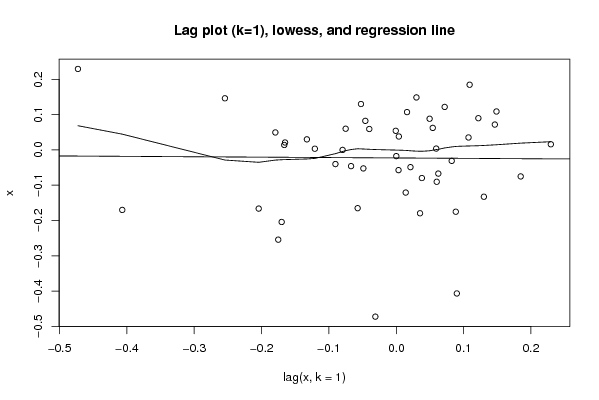
Figures (Output of Computation) | |||||||||||||||||||||||||||||||||||||||||||||||||||||
Input Parameters & R Code | |||||||||||||||||||||||||||||||||||||||||||||||||||||
| Parameters (Session): | |||||||||||||||||||||||||||||||||||||||||||||||||||||
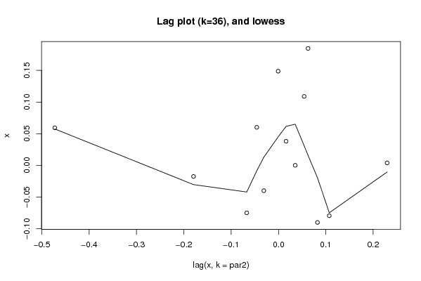
| par1 = 0 ; par2 = 36 ; | |||||||||||||||||||||||||||||||||||||||||||||||||||||
| Parameters (R input): | |||||||||||||||||||||||||||||||||||||||||||||||||||||
| par1 = 0 ; par2 = 36 ; | |||||||||||||||||||||||||||||||||||||||||||||||||||||
| R code (references can be found in the software module): | |||||||||||||||||||||||||||||||||||||||||||||||||||||
par1 <- as.numeric(par1) | |||||||||||||||||||||||||||||||||||||||||||||||||||||