Repository of Reproducible Computations

Free Statistics

of Irreproducible Research!

Author's title

Author

*The author of this computation has been verified*

R Software Module

rwasp_arimaforecasting.wasp

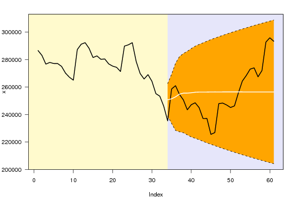
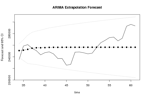
Title produced by software

ARIMA Forecasting

Date of computation

Fri, 11 Dec 2009 09:05:20 -0700

Cite this page as follows

Statistical Computations at FreeStatistics.org, Office for Research Development and Education, URL https://freestatistics.org/blog/index.php?v=date/2009/Dec/11/t1260547560esvd3mn32wwuw88.htm/, Retrieved Mon, 29 Apr 2024 02:44:45 +0000

Statistical Computations at FreeStatistics.org, Office for Research Development and Education, URL https://freestatistics.org/blog/index.php?pk=66443, Retrieved Mon, 29 Apr 2024 02:44:45 +0000

QR Codes:

Paste this QR Code to cite your computation.

Original text written by user:

IsPrivate?

No (this computation is public)

User-defined keywords

Estimated Impact

143

Family? (F = Feedback message, R = changed R code, M = changed R Module, P = changed Parameters, D = changed Data)

-     [ARIMA Forecasting] [] [2009-12-07 09:54:52] [b98453cac15ba1066b407e146608df68]
-   PD    [ARIMA Forecasting] [WS10] [2009-12-11 16:05:20] [40cfc51151e9382b81a5fb0c269b074d] [Current]
- RMP       [(Partial) Autocorrelation Function] [Verbetering works...] [2009-12-16 13:18:32] [7c2a5b25a196bd646844b8f5223c9b3e] 
- RMP       [(Partial) Autocorrelation Function] [Verbetering works...] [2009-12-16 13:24:30] [7c2a5b25a196bd646844b8f5223c9b3e] 
- RMP       [(Partial) Autocorrelation Function] [Verbetering works...] [2009-12-16 13:27:46] [7c2a5b25a196bd646844b8f5223c9b3e] 
- RMP       [(Partial) Autocorrelation Function] [Verbetering works...] [2009-12-16 13:27:46] [7c2a5b25a196bd646844b8f5223c9b3e] 
- RMP       [Variance Reduction Matrix] [Verbetering works...] [2009-12-16 13:31:53] [7c2a5b25a196bd646844b8f5223c9b3e] 
- RMP       [Spectral Analysis] [Verbetering works...] [2009-12-16 13:36:44] [7c2a5b25a196bd646844b8f5223c9b3e] 
- RMP       [Spectral Analysis] [Verbetering works...] [2009-12-16 13:41:05] [7c2a5b25a196bd646844b8f5223c9b3e] 
- RMP       [Standard Deviation-Mean Plot] [Verbetering works...] [2009-12-16 13:43:25] [7c2a5b25a196bd646844b8f5223c9b3e] 
- RMP       [ARIMA Backward Selection] [Verbetering works...] [2009-12-16 13:48:49] [7c2a5b25a196bd646844b8f5223c9b3e] 
-             [ARIMA Backward Selection] [Workshop 10] [2009-12-30 15:19:22] [90e6802d28d0afa9b030a19cd25ed2b0] 
- R P       [ARIMA Forecasting] [Verbetering works...] [2009-12-16 13:53:31] [7c2a5b25a196bd646844b8f5223c9b3e] 
-             [ARIMA Forecasting] [Workshop9] [2009-12-30 14:38:50] [90e6802d28d0afa9b030a19cd25ed2b0] 

Feedback Forum

Post a new message

Dataseries X:

Download CSV

Histogram

Boxplots

Summary of computational transaction
Raw Input	view raw input (R code)
Raw Output	view raw output of R engine
Computing time	3 seconds
R Server	'Gwilym Jenkins' @ 72.249.127.135

\begin{tabular}{lllllllll}
\hline
Summary of computational transaction \tabularnewline
Raw Input & view raw input (R code)  \tabularnewline
Raw Output & view raw output of R engine  \tabularnewline
Computing time & 3 seconds \tabularnewline
R Server & 'Gwilym Jenkins' @ 72.249.127.135 \tabularnewline
\hline
\end{tabular}
%Source: https://freestatistics.org/blog/index.php?pk=66443&T=0

[TABLE]
[ROW][C]Summary of computational transaction[/C][/ROW]
[ROW][C]Raw Input[/C][C]view raw input (R code) [/C][/ROW]
[ROW][C]Raw Output[/C][C]view raw output of R engine [/C][/ROW]
[ROW][C]Computing time[/C][C]3 seconds[/C][/ROW]
[ROW][C]R Server[/C][C]'Gwilym Jenkins' @ 72.249.127.135[/C][/ROW]
[/TABLE]
Source: https://freestatistics.org/blog/index.php?pk=66443&T=0

Globally Unique Identifier (entire table): ba.freestatistics.org/blog/index.php?pk=66443&T=0

As an alternative you can also use a QR Code:

The GUIDs for individual cells are displayed in the table below:

Summary of computational transaction
Raw Input	view raw input (R code)
Raw Output	view raw output of R engine
Computing time	3 seconds
R Server	'Gwilym Jenkins' @ 72.249.127.135

Univariate ARIMA Extrapolation Forecast
time	Y[t]	F[t]	95% LB	95% UB	p-value(H0: Y[t] = F[t])	P(F[t]>Y[t-1])	P(F[t]>Y[t-s])	P(F[t]>Y[33])
21	274352	-	-	-	-	-	-	-
22	271311	-	-	-	-	-	-	-
23	289802	-	-	-	-	-	-	-
24	290726	-	-	-	-	-	-	-
25	292300	-	-	-	-	-	-	-
26	278506	-	-	-	-	-	-	-
27	269826	-	-	-	-	-	-	-
28	265861	-	-	-	-	-	-	-
29	269034	-	-	-	-	-	-	-
30	264176	-	-	-	-	-	-	-
31	255198	-	-	-	-	-	-	-
32	253353	-	-	-	-	-	-	-
33	246057	-	-	-	-	-	-	-
34	235372	250718.8679	238946.2392	262491.4966	0.0053	0.7812	3e-04	0.7812
35	258556	251444.3868	233475.0347	269413.7389	0.219	0.9602	0	0.7216
36	260993	252858.2519	228423.4099	277293.094	0.257	0.3238	0.0012	0.7073
37	254663	254804.5182	227420.8425	282188.194	0.496	0.3289	0.0036	0.7344
38	250643	255574.1298	226751.0785	284397.181	0.3687	0.5247	0.0595	0.7412
39	243422	255592.7685	225169.4618	286016.0751	0.2165	0.6251	0.1796	0.7305
40	247105	255845.3132	223680.154	288010.4724	0.2972	0.7755	0.2708	0.7246
41	248541	256223.9897	222680.2249	289767.7545	0.3267	0.7029	0.2271	0.7238
42	245039	256346.8461	221652.7247	291040.9675	0.2615	0.6704	0.3291	0.7195
43	237080	256327.231	220462.4566	292192.0053	0.1464	0.7313	0.5246	0.7127
44	237085	256374.3155	219336.9551	293411.6759	0.1537	0.8464	0.5635	0.7075
45	225554	256449.1053	218324.5665	294573.6441	0.0561	0.8403	0.7034	0.7034
46	226839	256467.5838	217315.3193	295619.8484	0.069	0.9391	0.8545	0.6989
47	247934	256459.3304	216291.6887	296626.972	0.3387	0.9258	0.4593	0.6941
48	248333	256468.5685	215303.244	297633.8929	0.3492	0.6578	0.4147	0.69
49	246969	256483.5301	214354.0369	298613.0233	0.329	0.6477	0.5337	0.6862
50	245098	256485.9987	213419.0267	299552.9708	0.3021	0.6675	0.6048	0.6825
51	246263	256483.5428	212495.7904	300471.2951	0.3244	0.694	0.7197	0.6789
52	255765	256485.4539	211594.4246	301376.4832	0.4875	0.6723	0.6589	0.6756
53	264319	256488.4776	210714.046	302262.9092	0.3687	0.5124	0.6332	0.6724
54	268347	256488.7181	209848.5076	303128.9287	0.3091	0.3711	0.6848	0.6694
55	273046	256488.0774	208997.1174	303979.0373	0.2472	0.3123	0.7884	0.6666
56	273963	256488.4921	208161.5043	304815.4798	0.2393	0.2509	0.7843	0.6639
57	267430	256489.1076	207340.744	305637.4712	0.3313	0.2429	0.8913	0.6613
58	271993	256489.1024	206533.0206	306445.1842	0.2715	0.3339	0.8776	0.6588
59	292710	256488.9466	205737.8308	307240.0624	0.0809	0.2747	0.6294	0.6565
60	295881	256489.0401	204955.1095	308022.9707	0.067	0.0842	0.6218	0.6542
61	293299	256489.1659	204184.2272	308794.1047	0.0839	0.07	0.6394	0.6521

\begin{tabular}{lllllllll}
\hline
Univariate ARIMA Extrapolation Forecast \tabularnewline
time & Y[t] & F[t] & 95% LB & 95% UB & p-value(H0: Y[t] = F[t]) & P(F[t]>Y[t-1]) & P(F[t]>Y[t-s]) & P(F[t]>Y[33]) \tabularnewline
21 & 274352 & - & - & - & - & - & - & - \tabularnewline
22 & 271311 & - & - & - & - & - & - & - \tabularnewline
23 & 289802 & - & - & - & - & - & - & - \tabularnewline
24 & 290726 & - & - & - & - & - & - & - \tabularnewline
25 & 292300 & - & - & - & - & - & - & - \tabularnewline
26 & 278506 & - & - & - & - & - & - & - \tabularnewline
27 & 269826 & - & - & - & - & - & - & - \tabularnewline
28 & 265861 & - & - & - & - & - & - & - \tabularnewline
29 & 269034 & - & - & - & - & - & - & - \tabularnewline
30 & 264176 & - & - & - & - & - & - & - \tabularnewline
31 & 255198 & - & - & - & - & - & - & - \tabularnewline
32 & 253353 & - & - & - & - & - & - & - \tabularnewline
33 & 246057 & - & - & - & - & - & - & - \tabularnewline
34 & 235372 & 250718.8679 & 238946.2392 & 262491.4966 & 0.0053 & 0.7812 & 3e-04 & 0.7812 \tabularnewline
35 & 258556 & 251444.3868 & 233475.0347 & 269413.7389 & 0.219 & 0.9602 & 0 & 0.7216 \tabularnewline
36 & 260993 & 252858.2519 & 228423.4099 & 277293.094 & 0.257 & 0.3238 & 0.0012 & 0.7073 \tabularnewline
37 & 254663 & 254804.5182 & 227420.8425 & 282188.194 & 0.496 & 0.3289 & 0.0036 & 0.7344 \tabularnewline
38 & 250643 & 255574.1298 & 226751.0785 & 284397.181 & 0.3687 & 0.5247 & 0.0595 & 0.7412 \tabularnewline
39 & 243422 & 255592.7685 & 225169.4618 & 286016.0751 & 0.2165 & 0.6251 & 0.1796 & 0.7305 \tabularnewline
40 & 247105 & 255845.3132 & 223680.154 & 288010.4724 & 0.2972 & 0.7755 & 0.2708 & 0.7246 \tabularnewline
41 & 248541 & 256223.9897 & 222680.2249 & 289767.7545 & 0.3267 & 0.7029 & 0.2271 & 0.7238 \tabularnewline
42 & 245039 & 256346.8461 & 221652.7247 & 291040.9675 & 0.2615 & 0.6704 & 0.3291 & 0.7195 \tabularnewline
43 & 237080 & 256327.231 & 220462.4566 & 292192.0053 & 0.1464 & 0.7313 & 0.5246 & 0.7127 \tabularnewline
44 & 237085 & 256374.3155 & 219336.9551 & 293411.6759 & 0.1537 & 0.8464 & 0.5635 & 0.7075 \tabularnewline
45 & 225554 & 256449.1053 & 218324.5665 & 294573.6441 & 0.0561 & 0.8403 & 0.7034 & 0.7034 \tabularnewline
46 & 226839 & 256467.5838 & 217315.3193 & 295619.8484 & 0.069 & 0.9391 & 0.8545 & 0.6989 \tabularnewline
47 & 247934 & 256459.3304 & 216291.6887 & 296626.972 & 0.3387 & 0.9258 & 0.4593 & 0.6941 \tabularnewline
48 & 248333 & 256468.5685 & 215303.244 & 297633.8929 & 0.3492 & 0.6578 & 0.4147 & 0.69 \tabularnewline
49 & 246969 & 256483.5301 & 214354.0369 & 298613.0233 & 0.329 & 0.6477 & 0.5337 & 0.6862 \tabularnewline
50 & 245098 & 256485.9987 & 213419.0267 & 299552.9708 & 0.3021 & 0.6675 & 0.6048 & 0.6825 \tabularnewline
51 & 246263 & 256483.5428 & 212495.7904 & 300471.2951 & 0.3244 & 0.694 & 0.7197 & 0.6789 \tabularnewline
52 & 255765 & 256485.4539 & 211594.4246 & 301376.4832 & 0.4875 & 0.6723 & 0.6589 & 0.6756 \tabularnewline
53 & 264319 & 256488.4776 & 210714.046 & 302262.9092 & 0.3687 & 0.5124 & 0.6332 & 0.6724 \tabularnewline
54 & 268347 & 256488.7181 & 209848.5076 & 303128.9287 & 0.3091 & 0.3711 & 0.6848 & 0.6694 \tabularnewline
55 & 273046 & 256488.0774 & 208997.1174 & 303979.0373 & 0.2472 & 0.3123 & 0.7884 & 0.6666 \tabularnewline
56 & 273963 & 256488.4921 & 208161.5043 & 304815.4798 & 0.2393 & 0.2509 & 0.7843 & 0.6639 \tabularnewline
57 & 267430 & 256489.1076 & 207340.744 & 305637.4712 & 0.3313 & 0.2429 & 0.8913 & 0.6613 \tabularnewline
58 & 271993 & 256489.1024 & 206533.0206 & 306445.1842 & 0.2715 & 0.3339 & 0.8776 & 0.6588 \tabularnewline
59 & 292710 & 256488.9466 & 205737.8308 & 307240.0624 & 0.0809 & 0.2747 & 0.6294 & 0.6565 \tabularnewline
60 & 295881 & 256489.0401 & 204955.1095 & 308022.9707 & 0.067 & 0.0842 & 0.6218 & 0.6542 \tabularnewline
61 & 293299 & 256489.1659 & 204184.2272 & 308794.1047 & 0.0839 & 0.07 & 0.6394 & 0.6521 \tabularnewline
\hline
\end{tabular}
%Source: https://freestatistics.org/blog/index.php?pk=66443&T=1

[TABLE]
[ROW][C]Univariate ARIMA Extrapolation Forecast[/C][/ROW]
[ROW][C]time[/C][C]Y[t][/C][C]F[t][/C][C]95% LB[/C][C]95% UB[/C][C]p-value(H0: Y[t] = F[t])[/C][C]P(F[t]>Y[t-1])[/C][C]P(F[t]>Y[t-s])[/C][C]P(F[t]>Y[33])[/C][/ROW]
[ROW][C]21[/C][C]274352[/C][C]-[/C][C]-[/C][C]-[/C][C]-[/C][C]-[/C][C]-[/C][C]-[/C][/ROW]
[ROW][C]22[/C][C]271311[/C][C]-[/C][C]-[/C][C]-[/C][C]-[/C][C]-[/C][C]-[/C][C]-[/C][/ROW]
[ROW][C]23[/C][C]289802[/C][C]-[/C][C]-[/C][C]-[/C][C]-[/C][C]-[/C][C]-[/C][C]-[/C][/ROW]
[ROW][C]24[/C][C]290726[/C][C]-[/C][C]-[/C][C]-[/C][C]-[/C][C]-[/C][C]-[/C][C]-[/C][/ROW]
[ROW][C]25[/C][C]292300[/C][C]-[/C][C]-[/C][C]-[/C][C]-[/C][C]-[/C][C]-[/C][C]-[/C][/ROW]
[ROW][C]26[/C][C]278506[/C][C]-[/C][C]-[/C][C]-[/C][C]-[/C][C]-[/C][C]-[/C][C]-[/C][/ROW]
[ROW][C]27[/C][C]269826[/C][C]-[/C][C]-[/C][C]-[/C][C]-[/C][C]-[/C][C]-[/C][C]-[/C][/ROW]
[ROW][C]28[/C][C]265861[/C][C]-[/C][C]-[/C][C]-[/C][C]-[/C][C]-[/C][C]-[/C][C]-[/C][/ROW]
[ROW][C]29[/C][C]269034[/C][C]-[/C][C]-[/C][C]-[/C][C]-[/C][C]-[/C][C]-[/C][C]-[/C][/ROW]
[ROW][C]30[/C][C]264176[/C][C]-[/C][C]-[/C][C]-[/C][C]-[/C][C]-[/C][C]-[/C][C]-[/C][/ROW]
[ROW][C]31[/C][C]255198[/C][C]-[/C][C]-[/C][C]-[/C][C]-[/C][C]-[/C][C]-[/C][C]-[/C][/ROW]
[ROW][C]32[/C][C]253353[/C][C]-[/C][C]-[/C][C]-[/C][C]-[/C][C]-[/C][C]-[/C][C]-[/C][/ROW]
[ROW][C]33[/C][C]246057[/C][C]-[/C][C]-[/C][C]-[/C][C]-[/C][C]-[/C][C]-[/C][C]-[/C][/ROW]
[ROW][C]34[/C][C]235372[/C][C]250718.8679[/C][C]238946.2392[/C][C]262491.4966[/C][C]0.0053[/C][C]0.7812[/C][C]3e-04[/C][C]0.7812[/C][/ROW]
[ROW][C]35[/C][C]258556[/C][C]251444.3868[/C][C]233475.0347[/C][C]269413.7389[/C][C]0.219[/C][C]0.9602[/C][C]0[/C][C]0.7216[/C][/ROW]
[ROW][C]36[/C][C]260993[/C][C]252858.2519[/C][C]228423.4099[/C][C]277293.094[/C][C]0.257[/C][C]0.3238[/C][C]0.0012[/C][C]0.7073[/C][/ROW]
[ROW][C]37[/C][C]254663[/C][C]254804.5182[/C][C]227420.8425[/C][C]282188.194[/C][C]0.496[/C][C]0.3289[/C][C]0.0036[/C][C]0.7344[/C][/ROW]
[ROW][C]38[/C][C]250643[/C][C]255574.1298[/C][C]226751.0785[/C][C]284397.181[/C][C]0.3687[/C][C]0.5247[/C][C]0.0595[/C][C]0.7412[/C][/ROW]
[ROW][C]39[/C][C]243422[/C][C]255592.7685[/C][C]225169.4618[/C][C]286016.0751[/C][C]0.2165[/C][C]0.6251[/C][C]0.1796[/C][C]0.7305[/C][/ROW]
[ROW][C]40[/C][C]247105[/C][C]255845.3132[/C][C]223680.154[/C][C]288010.4724[/C][C]0.2972[/C][C]0.7755[/C][C]0.2708[/C][C]0.7246[/C][/ROW]
[ROW][C]41[/C][C]248541[/C][C]256223.9897[/C][C]222680.2249[/C][C]289767.7545[/C][C]0.3267[/C][C]0.7029[/C][C]0.2271[/C][C]0.7238[/C][/ROW]
[ROW][C]42[/C][C]245039[/C][C]256346.8461[/C][C]221652.7247[/C][C]291040.9675[/C][C]0.2615[/C][C]0.6704[/C][C]0.3291[/C][C]0.7195[/C][/ROW]
[ROW][C]43[/C][C]237080[/C][C]256327.231[/C][C]220462.4566[/C][C]292192.0053[/C][C]0.1464[/C][C]0.7313[/C][C]0.5246[/C][C]0.7127[/C][/ROW]
[ROW][C]44[/C][C]237085[/C][C]256374.3155[/C][C]219336.9551[/C][C]293411.6759[/C][C]0.1537[/C][C]0.8464[/C][C]0.5635[/C][C]0.7075[/C][/ROW]
[ROW][C]45[/C][C]225554[/C][C]256449.1053[/C][C]218324.5665[/C][C]294573.6441[/C][C]0.0561[/C][C]0.8403[/C][C]0.7034[/C][C]0.7034[/C][/ROW]
[ROW][C]46[/C][C]226839[/C][C]256467.5838[/C][C]217315.3193[/C][C]295619.8484[/C][C]0.069[/C][C]0.9391[/C][C]0.8545[/C][C]0.6989[/C][/ROW]
[ROW][C]47[/C][C]247934[/C][C]256459.3304[/C][C]216291.6887[/C][C]296626.972[/C][C]0.3387[/C][C]0.9258[/C][C]0.4593[/C][C]0.6941[/C][/ROW]
[ROW][C]48[/C][C]248333[/C][C]256468.5685[/C][C]215303.244[/C][C]297633.8929[/C][C]0.3492[/C][C]0.6578[/C][C]0.4147[/C][C]0.69[/C][/ROW]
[ROW][C]49[/C][C]246969[/C][C]256483.5301[/C][C]214354.0369[/C][C]298613.0233[/C][C]0.329[/C][C]0.6477[/C][C]0.5337[/C][C]0.6862[/C][/ROW]
[ROW][C]50[/C][C]245098[/C][C]256485.9987[/C][C]213419.0267[/C][C]299552.9708[/C][C]0.3021[/C][C]0.6675[/C][C]0.6048[/C][C]0.6825[/C][/ROW]
[ROW][C]51[/C][C]246263[/C][C]256483.5428[/C][C]212495.7904[/C][C]300471.2951[/C][C]0.3244[/C][C]0.694[/C][C]0.7197[/C][C]0.6789[/C][/ROW]
[ROW][C]52[/C][C]255765[/C][C]256485.4539[/C][C]211594.4246[/C][C]301376.4832[/C][C]0.4875[/C][C]0.6723[/C][C]0.6589[/C][C]0.6756[/C][/ROW]
[ROW][C]53[/C][C]264319[/C][C]256488.4776[/C][C]210714.046[/C][C]302262.9092[/C][C]0.3687[/C][C]0.5124[/C][C]0.6332[/C][C]0.6724[/C][/ROW]
[ROW][C]54[/C][C]268347[/C][C]256488.7181[/C][C]209848.5076[/C][C]303128.9287[/C][C]0.3091[/C][C]0.3711[/C][C]0.6848[/C][C]0.6694[/C][/ROW]
[ROW][C]55[/C][C]273046[/C][C]256488.0774[/C][C]208997.1174[/C][C]303979.0373[/C][C]0.2472[/C][C]0.3123[/C][C]0.7884[/C][C]0.6666[/C][/ROW]
[ROW][C]56[/C][C]273963[/C][C]256488.4921[/C][C]208161.5043[/C][C]304815.4798[/C][C]0.2393[/C][C]0.2509[/C][C]0.7843[/C][C]0.6639[/C][/ROW]
[ROW][C]57[/C][C]267430[/C][C]256489.1076[/C][C]207340.744[/C][C]305637.4712[/C][C]0.3313[/C][C]0.2429[/C][C]0.8913[/C][C]0.6613[/C][/ROW]
[ROW][C]58[/C][C]271993[/C][C]256489.1024[/C][C]206533.0206[/C][C]306445.1842[/C][C]0.2715[/C][C]0.3339[/C][C]0.8776[/C][C]0.6588[/C][/ROW]
[ROW][C]59[/C][C]292710[/C][C]256488.9466[/C][C]205737.8308[/C][C]307240.0624[/C][C]0.0809[/C][C]0.2747[/C][C]0.6294[/C][C]0.6565[/C][/ROW]
[ROW][C]60[/C][C]295881[/C][C]256489.0401[/C][C]204955.1095[/C][C]308022.9707[/C][C]0.067[/C][C]0.0842[/C][C]0.6218[/C][C]0.6542[/C][/ROW]
[ROW][C]61[/C][C]293299[/C][C]256489.1659[/C][C]204184.2272[/C][C]308794.1047[/C][C]0.0839[/C][C]0.07[/C][C]0.6394[/C][C]0.6521[/C][/ROW]
[/TABLE]
Source: https://freestatistics.org/blog/index.php?pk=66443&T=1

Globally Unique Identifier (entire table): ba.freestatistics.org/blog/index.php?pk=66443&T=1

As an alternative you can also use a QR Code:

The GUIDs for individual cells are displayed in the table below:

Univariate ARIMA Extrapolation Forecast
time	Y[t]	F[t]	95% LB	95% UB	p-value(H0: Y[t] = F[t])	P(F[t]>Y[t-1])	P(F[t]>Y[t-s])	P(F[t]>Y[33])
21	274352	-	-	-	-	-	-	-
22	271311	-	-	-	-	-	-	-
23	289802	-	-	-	-	-	-	-
24	290726	-	-	-	-	-	-	-
25	292300	-	-	-	-	-	-	-
26	278506	-	-	-	-	-	-	-
27	269826	-	-	-	-	-	-	-
28	265861	-	-	-	-	-	-	-
29	269034	-	-	-	-	-	-	-
30	264176	-	-	-	-	-	-	-
31	255198	-	-	-	-	-	-	-
32	253353	-	-	-	-	-	-	-
33	246057	-	-	-	-	-	-	-
34	235372	250718.8679	238946.2392	262491.4966	0.0053	0.7812	3e-04	0.7812
35	258556	251444.3868	233475.0347	269413.7389	0.219	0.9602	0	0.7216
36	260993	252858.2519	228423.4099	277293.094	0.257	0.3238	0.0012	0.7073
37	254663	254804.5182	227420.8425	282188.194	0.496	0.3289	0.0036	0.7344
38	250643	255574.1298	226751.0785	284397.181	0.3687	0.5247	0.0595	0.7412
39	243422	255592.7685	225169.4618	286016.0751	0.2165	0.6251	0.1796	0.7305
40	247105	255845.3132	223680.154	288010.4724	0.2972	0.7755	0.2708	0.7246
41	248541	256223.9897	222680.2249	289767.7545	0.3267	0.7029	0.2271	0.7238
42	245039	256346.8461	221652.7247	291040.9675	0.2615	0.6704	0.3291	0.7195
43	237080	256327.231	220462.4566	292192.0053	0.1464	0.7313	0.5246	0.7127
44	237085	256374.3155	219336.9551	293411.6759	0.1537	0.8464	0.5635	0.7075
45	225554	256449.1053	218324.5665	294573.6441	0.0561	0.8403	0.7034	0.7034
46	226839	256467.5838	217315.3193	295619.8484	0.069	0.9391	0.8545	0.6989
47	247934	256459.3304	216291.6887	296626.972	0.3387	0.9258	0.4593	0.6941
48	248333	256468.5685	215303.244	297633.8929	0.3492	0.6578	0.4147	0.69
49	246969	256483.5301	214354.0369	298613.0233	0.329	0.6477	0.5337	0.6862
50	245098	256485.9987	213419.0267	299552.9708	0.3021	0.6675	0.6048	0.6825
51	246263	256483.5428	212495.7904	300471.2951	0.3244	0.694	0.7197	0.6789
52	255765	256485.4539	211594.4246	301376.4832	0.4875	0.6723	0.6589	0.6756
53	264319	256488.4776	210714.046	302262.9092	0.3687	0.5124	0.6332	0.6724
54	268347	256488.7181	209848.5076	303128.9287	0.3091	0.3711	0.6848	0.6694
55	273046	256488.0774	208997.1174	303979.0373	0.2472	0.3123	0.7884	0.6666
56	273963	256488.4921	208161.5043	304815.4798	0.2393	0.2509	0.7843	0.6639
57	267430	256489.1076	207340.744	305637.4712	0.3313	0.2429	0.8913	0.6613
58	271993	256489.1024	206533.0206	306445.1842	0.2715	0.3339	0.8776	0.6588
59	292710	256488.9466	205737.8308	307240.0624	0.0809	0.2747	0.6294	0.6565
60	295881	256489.0401	204955.1095	308022.9707	0.067	0.0842	0.6218	0.6542
61	293299	256489.1659	204184.2272	308794.1047	0.0839	0.07	0.6394	0.6521

Univariate ARIMA Extrapolation Forecast Performance
time	% S.E.	PE	MAPE	Sq.E	MSE	RMSE
34	0.024	-0.0612	0	235526353.459	0	0
35	0.0365	0.0283	0.0447	50575042.738	143050698.0985	11960.3803
36	0.0493	0.0322	0.0406	66174126.2025	117425174.1331	10836.2897
37	0.0548	-6e-04	0.0306	20027.4051	88073887.4511	9384.7689
38	0.0575	-0.0193	0.0283	24316040.6256	75322318.086	8678.8431
39	0.0607	-0.0476	0.0315	148127604.7031	87456532.5222	9351.8197
40	0.0641	-0.0342	0.0319	76393075.3869	85876038.6457	9266.9325
41	0.0668	-0.03	0.0317	59028330.8248	82520075.1681	9084.0561
42	0.0691	-0.0441	0.033	127867383.3847	87558664.97	9357.2787
43	0.0714	-0.0751	0.0372	370455900.4964	115848388.5226	10763.2889
44	0.0737	-0.0752	0.0407	372077692.9879	139141961.6558	11795.8451
45	0.0758	-0.1205	0.0473	954507531.4424	207089092.4714	14390.5904
46	0.0779	-0.1155	0.0526	877852980.9054	258686314.6586	16083.7283
47	0.0799	-0.0332	0.0512	72681258.2701	245400239.2023	15665.2558
48	0.0819	-0.0317	0.0499	66187474.1963	233452721.5352	15279.1597
49	0.0838	-0.0371	0.0491	90526283.2824	224519819.1444	14983.9854
50	0.0857	-0.0444	0.0488	129686515.2729	218941389.5049	14796.6682
51	0.0875	-0.0398	0.0483	104459494.118	212581284.2056	14580.1675
52	0.0893	-0.0028	0.0459	519053.8449	201420114.1866	14192.2554
53	0.0911	0.0305	0.0452	61317080.9745	194414962.526	13943.2766
54	0.0928	0.0462	0.0452	140618848.6139	191853242.8159	13851.1098
55	0.0945	0.0646	0.0461	274164802.3399	195594677.3398	13985.5167
56	0.0961	0.0681	0.0471	305358427.1478	200367014.2879	14155.1056
57	0.0978	0.0427	0.0469	119703125.7093	197006018.9305	14035.8833
58	0.0994	0.0604	0.0474	240370840.17	198740611.7801	14097.5392
59	0.101	0.1412	0.051	1311964707.0683	241556923.1373	15542.1016
60	0.1025	0.1536	0.0548	1551726507.7359	290081722.5669	17031.7857
61	0.104	0.1435	0.058	1354963884.4213	328113228.3474	18113.896

\begin{tabular}{lllllllll}
\hline
Univariate ARIMA Extrapolation Forecast Performance \tabularnewline
time & % S.E. & PE & MAPE & Sq.E & MSE & RMSE \tabularnewline
34 & 0.024 & -0.0612 & 0 & 235526353.459 & 0 & 0 \tabularnewline
35 & 0.0365 & 0.0283 & 0.0447 & 50575042.738 & 143050698.0985 & 11960.3803 \tabularnewline
36 & 0.0493 & 0.0322 & 0.0406 & 66174126.2025 & 117425174.1331 & 10836.2897 \tabularnewline
37 & 0.0548 & -6e-04 & 0.0306 & 20027.4051 & 88073887.4511 & 9384.7689 \tabularnewline
38 & 0.0575 & -0.0193 & 0.0283 & 24316040.6256 & 75322318.086 & 8678.8431 \tabularnewline
39 & 0.0607 & -0.0476 & 0.0315 & 148127604.7031 & 87456532.5222 & 9351.8197 \tabularnewline
40 & 0.0641 & -0.0342 & 0.0319 & 76393075.3869 & 85876038.6457 & 9266.9325 \tabularnewline
41 & 0.0668 & -0.03 & 0.0317 & 59028330.8248 & 82520075.1681 & 9084.0561 \tabularnewline
42 & 0.0691 & -0.0441 & 0.033 & 127867383.3847 & 87558664.97 & 9357.2787 \tabularnewline
43 & 0.0714 & -0.0751 & 0.0372 & 370455900.4964 & 115848388.5226 & 10763.2889 \tabularnewline
44 & 0.0737 & -0.0752 & 0.0407 & 372077692.9879 & 139141961.6558 & 11795.8451 \tabularnewline
45 & 0.0758 & -0.1205 & 0.0473 & 954507531.4424 & 207089092.4714 & 14390.5904 \tabularnewline
46 & 0.0779 & -0.1155 & 0.0526 & 877852980.9054 & 258686314.6586 & 16083.7283 \tabularnewline
47 & 0.0799 & -0.0332 & 0.0512 & 72681258.2701 & 245400239.2023 & 15665.2558 \tabularnewline
48 & 0.0819 & -0.0317 & 0.0499 & 66187474.1963 & 233452721.5352 & 15279.1597 \tabularnewline
49 & 0.0838 & -0.0371 & 0.0491 & 90526283.2824 & 224519819.1444 & 14983.9854 \tabularnewline
50 & 0.0857 & -0.0444 & 0.0488 & 129686515.2729 & 218941389.5049 & 14796.6682 \tabularnewline
51 & 0.0875 & -0.0398 & 0.0483 & 104459494.118 & 212581284.2056 & 14580.1675 \tabularnewline
52 & 0.0893 & -0.0028 & 0.0459 & 519053.8449 & 201420114.1866 & 14192.2554 \tabularnewline
53 & 0.0911 & 0.0305 & 0.0452 & 61317080.9745 & 194414962.526 & 13943.2766 \tabularnewline
54 & 0.0928 & 0.0462 & 0.0452 & 140618848.6139 & 191853242.8159 & 13851.1098 \tabularnewline
55 & 0.0945 & 0.0646 & 0.0461 & 274164802.3399 & 195594677.3398 & 13985.5167 \tabularnewline
56 & 0.0961 & 0.0681 & 0.0471 & 305358427.1478 & 200367014.2879 & 14155.1056 \tabularnewline
57 & 0.0978 & 0.0427 & 0.0469 & 119703125.7093 & 197006018.9305 & 14035.8833 \tabularnewline
58 & 0.0994 & 0.0604 & 0.0474 & 240370840.17 & 198740611.7801 & 14097.5392 \tabularnewline
59 & 0.101 & 0.1412 & 0.051 & 1311964707.0683 & 241556923.1373 & 15542.1016 \tabularnewline
60 & 0.1025 & 0.1536 & 0.0548 & 1551726507.7359 & 290081722.5669 & 17031.7857 \tabularnewline
61 & 0.104 & 0.1435 & 0.058 & 1354963884.4213 & 328113228.3474 & 18113.896 \tabularnewline
\hline
\end{tabular}
%Source: https://freestatistics.org/blog/index.php?pk=66443&T=2

[TABLE]
[ROW][C]Univariate ARIMA Extrapolation Forecast Performance[/C][/ROW]
[ROW][C]time[/C][C]% S.E.[/C][C]PE[/C][C]MAPE[/C][C]Sq.E[/C][C]MSE[/C][C]RMSE[/C][/ROW]
[ROW][C]34[/C][C]0.024[/C][C]-0.0612[/C][C]0[/C][C]235526353.459[/C][C]0[/C][C]0[/C][/ROW]
[ROW][C]35[/C][C]0.0365[/C][C]0.0283[/C][C]0.0447[/C][C]50575042.738[/C][C]143050698.0985[/C][C]11960.3803[/C][/ROW]
[ROW][C]36[/C][C]0.0493[/C][C]0.0322[/C][C]0.0406[/C][C]66174126.2025[/C][C]117425174.1331[/C][C]10836.2897[/C][/ROW]
[ROW][C]37[/C][C]0.0548[/C][C]-6e-04[/C][C]0.0306[/C][C]20027.4051[/C][C]88073887.4511[/C][C]9384.7689[/C][/ROW]
[ROW][C]38[/C][C]0.0575[/C][C]-0.0193[/C][C]0.0283[/C][C]24316040.6256[/C][C]75322318.086[/C][C]8678.8431[/C][/ROW]
[ROW][C]39[/C][C]0.0607[/C][C]-0.0476[/C][C]0.0315[/C][C]148127604.7031[/C][C]87456532.5222[/C][C]9351.8197[/C][/ROW]
[ROW][C]40[/C][C]0.0641[/C][C]-0.0342[/C][C]0.0319[/C][C]76393075.3869[/C][C]85876038.6457[/C][C]9266.9325[/C][/ROW]
[ROW][C]41[/C][C]0.0668[/C][C]-0.03[/C][C]0.0317[/C][C]59028330.8248[/C][C]82520075.1681[/C][C]9084.0561[/C][/ROW]
[ROW][C]42[/C][C]0.0691[/C][C]-0.0441[/C][C]0.033[/C][C]127867383.3847[/C][C]87558664.97[/C][C]9357.2787[/C][/ROW]
[ROW][C]43[/C][C]0.0714[/C][C]-0.0751[/C][C]0.0372[/C][C]370455900.4964[/C][C]115848388.5226[/C][C]10763.2889[/C][/ROW]
[ROW][C]44[/C][C]0.0737[/C][C]-0.0752[/C][C]0.0407[/C][C]372077692.9879[/C][C]139141961.6558[/C][C]11795.8451[/C][/ROW]
[ROW][C]45[/C][C]0.0758[/C][C]-0.1205[/C][C]0.0473[/C][C]954507531.4424[/C][C]207089092.4714[/C][C]14390.5904[/C][/ROW]
[ROW][C]46[/C][C]0.0779[/C][C]-0.1155[/C][C]0.0526[/C][C]877852980.9054[/C][C]258686314.6586[/C][C]16083.7283[/C][/ROW]
[ROW][C]47[/C][C]0.0799[/C][C]-0.0332[/C][C]0.0512[/C][C]72681258.2701[/C][C]245400239.2023[/C][C]15665.2558[/C][/ROW]
[ROW][C]48[/C][C]0.0819[/C][C]-0.0317[/C][C]0.0499[/C][C]66187474.1963[/C][C]233452721.5352[/C][C]15279.1597[/C][/ROW]
[ROW][C]49[/C][C]0.0838[/C][C]-0.0371[/C][C]0.0491[/C][C]90526283.2824[/C][C]224519819.1444[/C][C]14983.9854[/C][/ROW]
[ROW][C]50[/C][C]0.0857[/C][C]-0.0444[/C][C]0.0488[/C][C]129686515.2729[/C][C]218941389.5049[/C][C]14796.6682[/C][/ROW]
[ROW][C]51[/C][C]0.0875[/C][C]-0.0398[/C][C]0.0483[/C][C]104459494.118[/C][C]212581284.2056[/C][C]14580.1675[/C][/ROW]
[ROW][C]52[/C][C]0.0893[/C][C]-0.0028[/C][C]0.0459[/C][C]519053.8449[/C][C]201420114.1866[/C][C]14192.2554[/C][/ROW]
[ROW][C]53[/C][C]0.0911[/C][C]0.0305[/C][C]0.0452[/C][C]61317080.9745[/C][C]194414962.526[/C][C]13943.2766[/C][/ROW]
[ROW][C]54[/C][C]0.0928[/C][C]0.0462[/C][C]0.0452[/C][C]140618848.6139[/C][C]191853242.8159[/C][C]13851.1098[/C][/ROW]
[ROW][C]55[/C][C]0.0945[/C][C]0.0646[/C][C]0.0461[/C][C]274164802.3399[/C][C]195594677.3398[/C][C]13985.5167[/C][/ROW]
[ROW][C]56[/C][C]0.0961[/C][C]0.0681[/C][C]0.0471[/C][C]305358427.1478[/C][C]200367014.2879[/C][C]14155.1056[/C][/ROW]
[ROW][C]57[/C][C]0.0978[/C][C]0.0427[/C][C]0.0469[/C][C]119703125.7093[/C][C]197006018.9305[/C][C]14035.8833[/C][/ROW]
[ROW][C]58[/C][C]0.0994[/C][C]0.0604[/C][C]0.0474[/C][C]240370840.17[/C][C]198740611.7801[/C][C]14097.5392[/C][/ROW]
[ROW][C]59[/C][C]0.101[/C][C]0.1412[/C][C]0.051[/C][C]1311964707.0683[/C][C]241556923.1373[/C][C]15542.1016[/C][/ROW]
[ROW][C]60[/C][C]0.1025[/C][C]0.1536[/C][C]0.0548[/C][C]1551726507.7359[/C][C]290081722.5669[/C][C]17031.7857[/C][/ROW]
[ROW][C]61[/C][C]0.104[/C][C]0.1435[/C][C]0.058[/C][C]1354963884.4213[/C][C]328113228.3474[/C][C]18113.896[/C][/ROW]
[/TABLE]
Source: https://freestatistics.org/blog/index.php?pk=66443&T=2

Globally Unique Identifier (entire table): ba.freestatistics.org/blog/index.php?pk=66443&T=2

As an alternative you can also use a QR Code:

The GUIDs for individual cells are displayed in the table below:

Univariate ARIMA Extrapolation Forecast Performance
time	% S.E.	PE	MAPE	Sq.E	MSE	RMSE
34	0.024	-0.0612	0	235526353.459	0	0
35	0.0365	0.0283	0.0447	50575042.738	143050698.0985	11960.3803
36	0.0493	0.0322	0.0406	66174126.2025	117425174.1331	10836.2897
37	0.0548	-6e-04	0.0306	20027.4051	88073887.4511	9384.7689
38	0.0575	-0.0193	0.0283	24316040.6256	75322318.086	8678.8431
39	0.0607	-0.0476	0.0315	148127604.7031	87456532.5222	9351.8197
40	0.0641	-0.0342	0.0319	76393075.3869	85876038.6457	9266.9325
41	0.0668	-0.03	0.0317	59028330.8248	82520075.1681	9084.0561
42	0.0691	-0.0441	0.033	127867383.3847	87558664.97	9357.2787
43	0.0714	-0.0751	0.0372	370455900.4964	115848388.5226	10763.2889
44	0.0737	-0.0752	0.0407	372077692.9879	139141961.6558	11795.8451
45	0.0758	-0.1205	0.0473	954507531.4424	207089092.4714	14390.5904
46	0.0779	-0.1155	0.0526	877852980.9054	258686314.6586	16083.7283
47	0.0799	-0.0332	0.0512	72681258.2701	245400239.2023	15665.2558
48	0.0819	-0.0317	0.0499	66187474.1963	233452721.5352	15279.1597
49	0.0838	-0.0371	0.0491	90526283.2824	224519819.1444	14983.9854
50	0.0857	-0.0444	0.0488	129686515.2729	218941389.5049	14796.6682
51	0.0875	-0.0398	0.0483	104459494.118	212581284.2056	14580.1675
52	0.0893	-0.0028	0.0459	519053.8449	201420114.1866	14192.2554
53	0.0911	0.0305	0.0452	61317080.9745	194414962.526	13943.2766
54	0.0928	0.0462	0.0452	140618848.6139	191853242.8159	13851.1098
55	0.0945	0.0646	0.0461	274164802.3399	195594677.3398	13985.5167
56	0.0961	0.0681	0.0471	305358427.1478	200367014.2879	14155.1056
57	0.0978	0.0427	0.0469	119703125.7093	197006018.9305	14035.8833
58	0.0994	0.0604	0.0474	240370840.17	198740611.7801	14097.5392
59	0.101	0.1412	0.051	1311964707.0683	241556923.1373	15542.1016
60	0.1025	0.1536	0.0548	1551726507.7359	290081722.5669	17031.7857
61	0.104	0.1435	0.058	1354963884.4213	328113228.3474	18113.896

Figure 1

PNG link

Postscript link

PDF link

Figure 2

PNG link

Postscript link

PDF link

Parameters (Session):

par1 = 24 ; par2 = 1 ; par3 = 1 ; par4 = 0 ; par5 = 12 ; par6 = 0 ; par7 = 0 ; par8 = 0 ; par9 = 0 ; par10 = FALSE ;

Parameters (R input):

par1 = 24 ; par2 = 1 ; par3 = 1 ; par4 = 0 ; par5 = 12 ; par6 = 0 ; par7 = 0 ; par8 = 0 ; par9 = 0 ; par10 = FALSE ;

R code (references can be found in the software module):

par1 <- as.numeric(par1) #cut off periods
par1 <- 28
par2 <- as.numeric(par2) #lambda
par3 <- as.numeric(par3) #degree of non-seasonal differencing
par4 <- as.numeric(par4) #degree of seasonal differencing
par5 <- as.numeric(par5) #seasonal period
par6 <- as.numeric(par6) #p
par6 <- 3
par7 <- as.numeric(par7) #q
par7 <- 3
par8 <- as.numeric(par8) #P
par9 <- as.numeric(par9) #Q
if (par10 == 'TRUE') par10 <- TRUE
if (par10 == 'FALSE') par10 <- FALSE
if (par2 == 0) x <- log(x)
if (par2 != 0) x <- x^par2
lx <- length(x)
first <- lx - 2*par1
nx <- lx - par1
nx1 <- nx + 1
fx <- lx - nx
if (fx < 1) {
fx <- par5
nx1 <- lx + fx - 1
first <- lx - 2*fx
}
first <- 1
if (fx < 3) fx <- round(lx/10,0)
(arima.out <- arima(x[1:nx], order=c(par6,par3,par7), seasonal=list(order=c(par8,par4,par9), period=par5), include.mean=par10, method='ML'))
(forecast <- predict(arima.out,par1))
(lb <- forecast$pred - 1.96 * forecast$se)
(ub <- forecast$pred + 1.96 * forecast$se)
if (par2 == 0) {
x <- exp(x)
forecast$pred <- exp(forecast$pred)
lb <- exp(lb)
ub <- exp(ub)
}
if (par2 != 0) {
x <- x^(1/par2)
forecast$pred <- forecast$pred^(1/par2)
lb <- lb^(1/par2)
ub <- ub^(1/par2)
}
if (par2 < 0) {
olb <- lb
lb <- ub
ub <- olb
}
(actandfor <- c(x[1:nx], forecast$pred))
(perc.se <- (ub-forecast$pred)/1.96/forecast$pred)
bitmap(file='test1.png')
opar <- par(mar=c(4,4,2,2),las=1)
ylim <- c( min(x[first:nx],lb), max(x[first:nx],ub))
plot(x,ylim=ylim,type='n',xlim=c(first,lx))
usr <- par('usr')
rect(usr[1],usr[3],nx+1,usr[4],border=NA,col='lemonchiffon')
rect(nx1,usr[3],usr[2],usr[4],border=NA,col='lavender')
abline(h= (-3:3)*2 , col ='gray', lty =3)
polygon( c(nx1:lx,lx:nx1), c(lb,rev(ub)), col = 'orange', lty=2,border=NA)
lines(nx1:lx, lb , lty=2)
lines(nx1:lx, ub , lty=2)
lines(x, lwd=2)
lines(nx1:lx, forecast$pred , lwd=2 , col ='white')
box()
par(opar)
dev.off()
prob.dec <- array(NA, dim=fx)
prob.sdec <- array(NA, dim=fx)
prob.ldec <- array(NA, dim=fx)
prob.pval <- array(NA, dim=fx)
perf.pe <- array(0, dim=fx)
perf.mape <- array(0, dim=fx)
perf.mape1 <- array(0, dim=fx)
perf.se <- array(0, dim=fx)
perf.mse <- array(0, dim=fx)
perf.mse1 <- array(0, dim=fx)
perf.rmse <- array(0, dim=fx)
for (i in 1:fx) {
locSD <- (ub[i] - forecast$pred[i]) / 1.96
perf.pe[i] = (x[nx+i] - forecast$pred[i]) / forecast$pred[i]
perf.se[i] = (x[nx+i] - forecast$pred[i])^2
prob.dec[i] = pnorm((x[nx+i-1] - forecast$pred[i]) / locSD)
prob.sdec[i] = pnorm((x[nx+i-par5] - forecast$pred[i]) / locSD)
prob.ldec[i] = pnorm((x[nx] - forecast$pred[i]) / locSD)
prob.pval[i] = pnorm(abs(x[nx+i] - forecast$pred[i]) / locSD)
}
perf.mape[1] = abs(perf.pe[1])
perf.mse[1] = abs(perf.se[1])
for (i in 2:fx) {
perf.mape[i] = perf.mape[i-1] + abs(perf.pe[i])
perf.mape1[i] = perf.mape[i] / i
perf.mse[i] = perf.mse[i-1] + perf.se[i]
perf.mse1[i] = perf.mse[i] / i
}
perf.rmse = sqrt(perf.mse1)
bitmap(file='test2.png')
plot(forecast$pred, pch=19, type='b',main='ARIMA Extrapolation Forecast', ylab='Forecast and 95% CI', xlab='time',ylim=c(min(lb),max(ub)))
dum <- forecast$pred
dum[1:par1] <- x[(nx+1):lx]
lines(dum, lty=1)
lines(ub,lty=3)
lines(lb,lty=3)
dev.off()
load(file='createtable')
a<-table.start()
a<-table.row.start(a)
a<-table.element(a,'Univariate ARIMA Extrapolation Forecast',9,TRUE)
a<-table.row.end(a)
a<-table.row.start(a)
a<-table.element(a,'time',1,header=TRUE)
a<-table.element(a,'Y[t]',1,header=TRUE)
a<-table.element(a,'F[t]',1,header=TRUE)
a<-table.element(a,'95% LB',1,header=TRUE)
a<-table.element(a,'95% UB',1,header=TRUE)
a<-table.element(a,'p-value
(H0: Y[t] = F[t])',1,header=TRUE)
a<-table.element(a,'P(F[t]>Y[t-1])',1,header=TRUE)
a<-table.element(a,'P(F[t]>Y[t-s])',1,header=TRUE)
mylab <- paste('P(F[t]>Y[',nx,sep='')
mylab <- paste(mylab,'])',sep='')
a<-table.element(a,mylab,1,header=TRUE)
a<-table.row.end(a)
for (i in (nx-par5):nx) {
a<-table.row.start(a)
a<-table.element(a,i,header=TRUE)
a<-table.element(a,x[i])
a<-table.element(a,'-')
a<-table.element(a,'-')
a<-table.element(a,'-')
a<-table.element(a,'-')
a<-table.element(a,'-')
a<-table.element(a,'-')
a<-table.element(a,'-')
a<-table.row.end(a)
}
for (i in 1:fx) {
a<-table.row.start(a)
a<-table.element(a,nx+i,header=TRUE)
a<-table.element(a,round(x[nx+i],4))
a<-table.element(a,round(forecast$pred[i],4))
a<-table.element(a,round(lb[i],4))
a<-table.element(a,round(ub[i],4))
a<-table.element(a,round((1-prob.pval[i]),4))
a<-table.element(a,round((1-prob.dec[i]),4))
a<-table.element(a,round((1-prob.sdec[i]),4))
a<-table.element(a,round((1-prob.ldec[i]),4))
a<-table.row.end(a)
}
a<-table.end(a)
table.save(a,file='mytable.tab')
a<-table.start()
a<-table.row.start(a)
a<-table.element(a,'Univariate ARIMA Extrapolation Forecast Performance',7,TRUE)
a<-table.row.end(a)
a<-table.row.start(a)
a<-table.element(a,'time',1,header=TRUE)
a<-table.element(a,'% S.E.',1,header=TRUE)
a<-table.element(a,'PE',1,header=TRUE)
a<-table.element(a,'MAPE',1,header=TRUE)
a<-table.element(a,'Sq.E',1,header=TRUE)
a<-table.element(a,'MSE',1,header=TRUE)
a<-table.element(a,'RMSE',1,header=TRUE)
a<-table.row.end(a)
for (i in 1:fx) {
a<-table.row.start(a)
a<-table.element(a,nx+i,header=TRUE)
a<-table.element(a,round(perc.se[i],4))
a<-table.element(a,round(perf.pe[i],4))
a<-table.element(a,round(perf.mape1[i],4))
a<-table.element(a,round(perf.se[i],4))
a<-table.element(a,round(perf.mse1[i],4))
a<-table.element(a,round(perf.rmse[i],4))
a<-table.row.end(a)
}
a<-table.end(a)
table.save(a,file='mytable1.tab')

Free Statistics

Description of Statistical Computation

Tree of Dependent Computations

Dataset

Tables (Output of Computation)

Figures (Output of Computation)

Input Parameters & R Code