Free Statistics
of Irreproducible Research!
Description of Statistical Computation | |||||||||||||||||||||||||||||||||||||||||||||||||||||
|---|---|---|---|---|---|---|---|---|---|---|---|---|---|---|---|---|---|---|---|---|---|---|---|---|---|---|---|---|---|---|---|---|---|---|---|---|---|---|---|---|---|---|---|---|---|---|---|---|---|---|---|---|---|
| Author's title | |||||||||||||||||||||||||||||||||||||||||||||||||||||
| Author | *The author of this computation has been verified* | ||||||||||||||||||||||||||||||||||||||||||||||||||||
| R Software Module | rwasp_edauni.wasp | ||||||||||||||||||||||||||||||||||||||||||||||||||||
| Title produced by software | Univariate Explorative Data Analysis | ||||||||||||||||||||||||||||||||||||||||||||||||||||
| Date of computation | Fri, 11 Dec 2009 06:29:26 -0700 | ||||||||||||||||||||||||||||||||||||||||||||||||||||
| Cite this page as follows | Statistical Computations at FreeStatistics.org, Office for Research Development and Education, URL https://freestatistics.org/blog/index.php?v=date/2009/Dec/11/t1260538208a51kq9atfzxsdpa.htm/, Retrieved Mon, 29 Apr 2024 02:24:03 +0000 | ||||||||||||||||||||||||||||||||||||||||||||||||||||
| Statistical Computations at FreeStatistics.org, Office for Research Development and Education, URL https://freestatistics.org/blog/index.php?pk=66179, Retrieved Mon, 29 Apr 2024 02:24:03 +0000 | |||||||||||||||||||||||||||||||||||||||||||||||||||||
| QR Codes: | |||||||||||||||||||||||||||||||||||||||||||||||||||||
|
| |||||||||||||||||||||||||||||||||||||||||||||||||||||
| Original text written by user: | |||||||||||||||||||||||||||||||||||||||||||||||||||||
| IsPrivate? | No (this computation is public) | ||||||||||||||||||||||||||||||||||||||||||||||||||||
| User-defined keywords | |||||||||||||||||||||||||||||||||||||||||||||||||||||
| Estimated Impact | 136 | ||||||||||||||||||||||||||||||||||||||||||||||||||||
Tree of Dependent Computations | |||||||||||||||||||||||||||||||||||||||||||||||||||||
| Family? (F = Feedback message, R = changed R code, M = changed R Module, P = changed Parameters, D = changed Data) | |||||||||||||||||||||||||||||||||||||||||||||||||||||
| - [Bivariate Data Series] [Bivariate dataset] [2008-01-05 23:51:08] [74be16979710d4c4e7c6647856088456] F RMPD [Univariate Explorative Data Analysis] [Colombia Coffee] [2008-01-07 14:21:11] [74be16979710d4c4e7c6647856088456] F RMPD [Univariate Data Series] [] [2009-10-14 08:30:28] [74be16979710d4c4e7c6647856088456] - RMP [Univariate Explorative Data Analysis] [WS3] [2009-10-19 07:33:07] [eaf42bcf5162b5692bb3c7f9d4636222] - M D [Univariate Explorative Data Analysis] [paper assumpties ...] [2009-12-11 13:29:26] [78d370e6d5f4594e9982a5085e7604c6] [Current] - RMP [Central Tendency] [paper assumpties ...] [2009-12-11 14:14:56] [eaf42bcf5162b5692bb3c7f9d4636222] - D [Univariate Explorative Data Analysis] [paper assumpties ...] [2009-12-11 14:38:50] [eaf42bcf5162b5692bb3c7f9d4636222] | |||||||||||||||||||||||||||||||||||||||||||||||||||||
| Feedback Forum | |||||||||||||||||||||||||||||||||||||||||||||||||||||
Post a new message | |||||||||||||||||||||||||||||||||||||||||||||||||||||
Dataset | |||||||||||||||||||||||||||||||||||||||||||||||||||||
| Dataseries X: | |||||||||||||||||||||||||||||||||||||||||||||||||||||
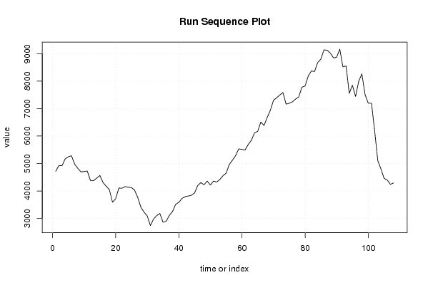
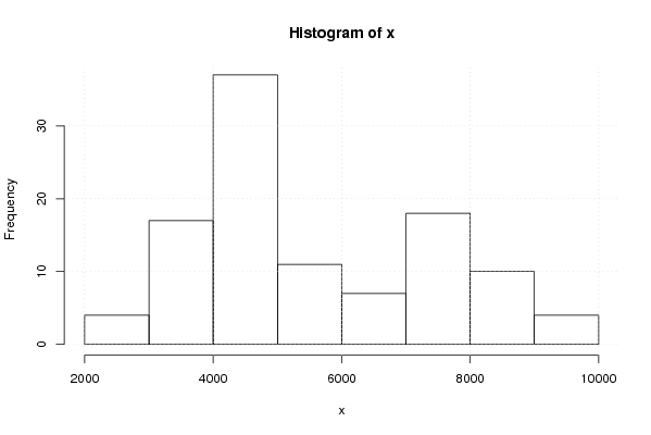
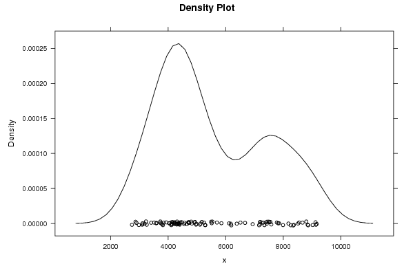
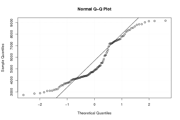
4716.99 4926.65 4920.10 5170.09 5246.24 5283.61 4979.05 4825.20 4695.12 4711.54 4727.22 4384.96 4378.75 4472.93 4564.07 4310.54 4171.38 4049.38 3591.37 3720.46 4107.23 4101.71 4162.34 4136.22 4125.88 4031.48 3761.36 3408.56 3228.47 3090.45 2741.14 2980.44 3104.33 3181.57 2863.86 2898.01 3112.33 3254.33 3513.47 3587.61 3727.45 3793.34 3817.58 3845.13 3931.86 4197.52 4307.13 4229.43 4362.28 4217.34 4361.28 4327.74 4417.65 4557.68 4650.35 4967.18 5123.42 5290.85 5535.66 5514.06 5493.88 5694.83 5850.41 6116.64 6175.00 6513.58 6383.78 6673.66 6936.61 7300.68 7392.93 7497.31 7584.71 7160.79 7196.19 7245.63 7347.51 7425.75 7778.51 7822.33 8181.22 8371.47 8347.71 8672.11 8802.79 9138.46 9123.29 9023.21 8850.41 8864.58 9163.74 8516.66 8553.44 7555.20 7851.22 7442.00 7992.53 8264.04 7517.39 7200.40 7193.69 6193.58 5104.21 4800.46 4461.61 4398.59 4243.63 4293.82 | |||||||||||||||||||||||||||||||||||||||||||||||||||||
Tables (Output of Computation) | |||||||||||||||||||||||||||||||||||||||||||||||||||||
| |||||||||||||||||||||||||||||||||||||||||||||||||||||
Figures (Output of Computation) | |||||||||||||||||||||||||||||||||||||||||||||||||||||
Input Parameters & R Code | |||||||||||||||||||||||||||||||||||||||||||||||||||||
| Parameters (Session): | |||||||||||||||||||||||||||||||||||||||||||||||||||||
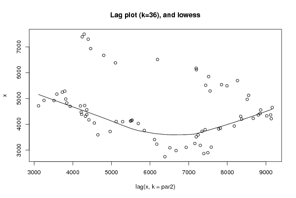
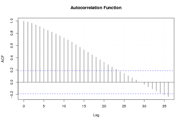
| par1 = 0 ; par2 = 36 ; | |||||||||||||||||||||||||||||||||||||||||||||||||||||
| Parameters (R input): | |||||||||||||||||||||||||||||||||||||||||||||||||||||
| par1 = 0 ; par2 = 36 ; | |||||||||||||||||||||||||||||||||||||||||||||||||||||
| R code (references can be found in the software module): | |||||||||||||||||||||||||||||||||||||||||||||||||||||
par1 <- as.numeric(par1) | |||||||||||||||||||||||||||||||||||||||||||||||||||||