Repository of Reproducible Computations

Free Statistics

of Irreproducible Research!

Author's title

Author

*Unverified author*

R Software Module

rwasp_autocorrelation.wasp

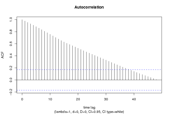
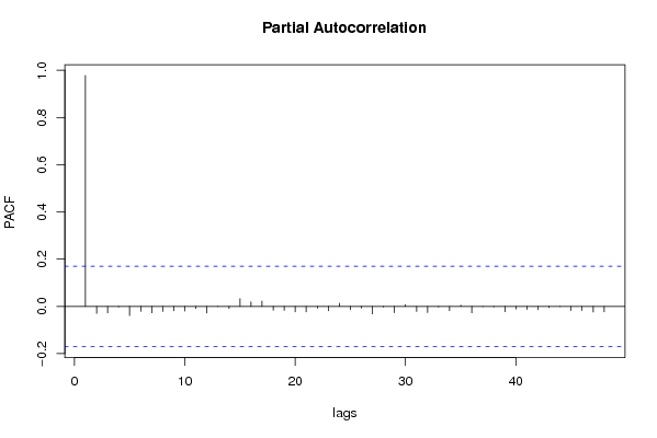
Title produced by software

(Partial) Autocorrelation Function

Date of computation

Wed, 09 Dec 2009 23:24:12 -0700

Cite this page as follows

Statistical Computations at FreeStatistics.org, Office for Research Development and Education, URL https://freestatistics.org/blog/index.php?v=date/2009/Dec/10/t1260426311olbmryfr2d7gbh7.htm/, Retrieved Sat, 27 Apr 2024 00:30:36 +0000

Statistical Computations at FreeStatistics.org, Office for Research Development and Education, URL https://freestatistics.org/blog/index.php?pk=65225, Retrieved Sat, 27 Apr 2024 00:30:36 +0000

QR Codes:

Paste this QR Code to cite your computation.

Original text written by user:

IsPrivate?

No (this computation is public)

User-defined keywords

KDGP2W21

Estimated Impact

162

Family? (F = Feedback message, R = changed R code, M = changed R Module, P = changed Parameters, D = changed Data)

-       [(Partial) Autocorrelation Function] [opgave 6bis oefen...] [2009-12-10 06:24:12] [712c3abbba27b8add982e356cd7e4c7f] [Current]

Feedback Forum

Post a new message

Dataseries X:

Download CSV

Histogram

Boxplots

Summary of computational transaction
Raw Input	view raw input (R code)
Raw Output	view raw output of R engine
Computing time	1 seconds
R Server	'Gwilym Jenkins' @ 72.249.127.135

\begin{tabular}{lllllllll}
\hline
Summary of computational transaction \tabularnewline
Raw Input & view raw input (R code)  \tabularnewline
Raw Output & view raw output of R engine  \tabularnewline
Computing time & 1 seconds \tabularnewline
R Server & 'Gwilym Jenkins' @ 72.249.127.135 \tabularnewline
\hline
\end{tabular}
%Source: https://freestatistics.org/blog/index.php?pk=65225&T=0

[TABLE]
[ROW][C]Summary of computational transaction[/C][/ROW]
[ROW][C]Raw Input[/C][C]view raw input (R code) [/C][/ROW]
[ROW][C]Raw Output[/C][C]view raw output of R engine [/C][/ROW]
[ROW][C]Computing time[/C][C]1 seconds[/C][/ROW]
[ROW][C]R Server[/C][C]'Gwilym Jenkins' @ 72.249.127.135[/C][/ROW]
[/TABLE]
Source: https://freestatistics.org/blog/index.php?pk=65225&T=0

Globally Unique Identifier (entire table): ba.freestatistics.org/blog/index.php?pk=65225&T=0

As an alternative you can also use a QR Code:

The GUIDs for individual cells are displayed in the table below:

Summary of computational transaction
Raw Input	view raw input (R code)
Raw Output	view raw output of R engine
Computing time	1 seconds
R Server	'Gwilym Jenkins' @ 72.249.127.135

Autocorrelation Function
Time lag k	ACF(k)	T-STAT	P-value
1	0.978001	11.2364	0
2	0.955198	10.9744	0
3	0.931707	10.7045	0
4	0.908618	10.4392	0
5	0.884382	10.1608	0
6	0.85978	9.8781	0
7	0.834532	9.588	0
8	0.808949	9.2941	0
9	0.783128	8.9975	0
10	0.757064	8.698	0
11	0.731244	8.4014	0
12	0.704853	8.0981	0
13	0.679089	7.8021	0
14	0.653612	7.5094	0
15	0.630264	7.2412	0
16	0.6084	6.99	0
17	0.588241	6.7584	0
18	0.56799	6.5257	0
19	0.547715	6.2928	0
20	0.527109	6.056	0
21	0.506269	5.8166	0
22	0.485801	5.5814	0
23	0.465243	5.3452	0
24	0.44596	5.1237	1e-06
25	0.426684	4.9022	1e-06
26	0.407766	4.6849	3e-06
27	0.388021	4.458	9e-06
28	0.368853	4.2378	2.1e-05
29	0.34902	4.0099	5.1e-05
30	0.330087	3.7924	0.000113
31	0.31065	3.5691	0.00025
32	0.290708	3.34	0.000545
33	0.271261	3.1165	0.001123
34	0.25182	2.8932	0.002231
35	0.233377	2.6813	0.004135
36	0.214424	2.4635	0.007522
37	0.19615	2.2536	0.012936
38	0.178282	2.0483	0.021256
39	0.160179	1.8403	0.033984
40	0.142128	1.6329	0.052433
41	0.124376	1.429	0.077687
42	0.106746	1.2264	0.111112
43	0.089722	1.0308	0.152254
44	0.073389	0.8432	0.200329
45	0.05706	0.6556	0.256621
46	0.040745	0.4681	0.320233
47	0.024094	0.2768	0.391175
48	0.007276	0.0836	0.466752

\begin{tabular}{lllllllll}
\hline
Autocorrelation Function \tabularnewline
Time lag k & ACF(k) & T-STAT & P-value \tabularnewline
1 & 0.978001 & 11.2364 & 0 \tabularnewline
2 & 0.955198 & 10.9744 & 0 \tabularnewline
3 & 0.931707 & 10.7045 & 0 \tabularnewline
4 & 0.908618 & 10.4392 & 0 \tabularnewline
5 & 0.884382 & 10.1608 & 0 \tabularnewline
6 & 0.85978 & 9.8781 & 0 \tabularnewline
7 & 0.834532 & 9.588 & 0 \tabularnewline
8 & 0.808949 & 9.2941 & 0 \tabularnewline
9 & 0.783128 & 8.9975 & 0 \tabularnewline
10 & 0.757064 & 8.698 & 0 \tabularnewline
11 & 0.731244 & 8.4014 & 0 \tabularnewline
12 & 0.704853 & 8.0981 & 0 \tabularnewline
13 & 0.679089 & 7.8021 & 0 \tabularnewline
14 & 0.653612 & 7.5094 & 0 \tabularnewline
15 & 0.630264 & 7.2412 & 0 \tabularnewline
16 & 0.6084 & 6.99 & 0 \tabularnewline
17 & 0.588241 & 6.7584 & 0 \tabularnewline
18 & 0.56799 & 6.5257 & 0 \tabularnewline
19 & 0.547715 & 6.2928 & 0 \tabularnewline
20 & 0.527109 & 6.056 & 0 \tabularnewline
21 & 0.506269 & 5.8166 & 0 \tabularnewline
22 & 0.485801 & 5.5814 & 0 \tabularnewline
23 & 0.465243 & 5.3452 & 0 \tabularnewline
24 & 0.44596 & 5.1237 & 1e-06 \tabularnewline
25 & 0.426684 & 4.9022 & 1e-06 \tabularnewline
26 & 0.407766 & 4.6849 & 3e-06 \tabularnewline
27 & 0.388021 & 4.458 & 9e-06 \tabularnewline
28 & 0.368853 & 4.2378 & 2.1e-05 \tabularnewline
29 & 0.34902 & 4.0099 & 5.1e-05 \tabularnewline
30 & 0.330087 & 3.7924 & 0.000113 \tabularnewline
31 & 0.31065 & 3.5691 & 0.00025 \tabularnewline
32 & 0.290708 & 3.34 & 0.000545 \tabularnewline
33 & 0.271261 & 3.1165 & 0.001123 \tabularnewline
34 & 0.25182 & 2.8932 & 0.002231 \tabularnewline
35 & 0.233377 & 2.6813 & 0.004135 \tabularnewline
36 & 0.214424 & 2.4635 & 0.007522 \tabularnewline
37 & 0.19615 & 2.2536 & 0.012936 \tabularnewline
38 & 0.178282 & 2.0483 & 0.021256 \tabularnewline
39 & 0.160179 & 1.8403 & 0.033984 \tabularnewline
40 & 0.142128 & 1.6329 & 0.052433 \tabularnewline
41 & 0.124376 & 1.429 & 0.077687 \tabularnewline
42 & 0.106746 & 1.2264 & 0.111112 \tabularnewline
43 & 0.089722 & 1.0308 & 0.152254 \tabularnewline
44 & 0.073389 & 0.8432 & 0.200329 \tabularnewline
45 & 0.05706 & 0.6556 & 0.256621 \tabularnewline
46 & 0.040745 & 0.4681 & 0.320233 \tabularnewline
47 & 0.024094 & 0.2768 & 0.391175 \tabularnewline
48 & 0.007276 & 0.0836 & 0.466752 \tabularnewline
\hline
\end{tabular}
%Source: https://freestatistics.org/blog/index.php?pk=65225&T=1

[TABLE]
[ROW][C]Autocorrelation Function[/C][/ROW]
[ROW][C]Time lag k[/C][C]ACF(k)[/C][C]T-STAT[/C][C]P-value[/C][/ROW]
[ROW][C]1[/C][C]0.978001[/C][C]11.2364[/C][C]0[/C][/ROW]
[ROW][C]2[/C][C]0.955198[/C][C]10.9744[/C][C]0[/C][/ROW]
[ROW][C]3[/C][C]0.931707[/C][C]10.7045[/C][C]0[/C][/ROW]
[ROW][C]4[/C][C]0.908618[/C][C]10.4392[/C][C]0[/C][/ROW]
[ROW][C]5[/C][C]0.884382[/C][C]10.1608[/C][C]0[/C][/ROW]
[ROW][C]6[/C][C]0.85978[/C][C]9.8781[/C][C]0[/C][/ROW]
[ROW][C]7[/C][C]0.834532[/C][C]9.588[/C][C]0[/C][/ROW]
[ROW][C]8[/C][C]0.808949[/C][C]9.2941[/C][C]0[/C][/ROW]
[ROW][C]9[/C][C]0.783128[/C][C]8.9975[/C][C]0[/C][/ROW]
[ROW][C]10[/C][C]0.757064[/C][C]8.698[/C][C]0[/C][/ROW]
[ROW][C]11[/C][C]0.731244[/C][C]8.4014[/C][C]0[/C][/ROW]
[ROW][C]12[/C][C]0.704853[/C][C]8.0981[/C][C]0[/C][/ROW]
[ROW][C]13[/C][C]0.679089[/C][C]7.8021[/C][C]0[/C][/ROW]
[ROW][C]14[/C][C]0.653612[/C][C]7.5094[/C][C]0[/C][/ROW]
[ROW][C]15[/C][C]0.630264[/C][C]7.2412[/C][C]0[/C][/ROW]
[ROW][C]16[/C][C]0.6084[/C][C]6.99[/C][C]0[/C][/ROW]
[ROW][C]17[/C][C]0.588241[/C][C]6.7584[/C][C]0[/C][/ROW]
[ROW][C]18[/C][C]0.56799[/C][C]6.5257[/C][C]0[/C][/ROW]
[ROW][C]19[/C][C]0.547715[/C][C]6.2928[/C][C]0[/C][/ROW]
[ROW][C]20[/C][C]0.527109[/C][C]6.056[/C][C]0[/C][/ROW]
[ROW][C]21[/C][C]0.506269[/C][C]5.8166[/C][C]0[/C][/ROW]
[ROW][C]22[/C][C]0.485801[/C][C]5.5814[/C][C]0[/C][/ROW]
[ROW][C]23[/C][C]0.465243[/C][C]5.3452[/C][C]0[/C][/ROW]
[ROW][C]24[/C][C]0.44596[/C][C]5.1237[/C][C]1e-06[/C][/ROW]
[ROW][C]25[/C][C]0.426684[/C][C]4.9022[/C][C]1e-06[/C][/ROW]
[ROW][C]26[/C][C]0.407766[/C][C]4.6849[/C][C]3e-06[/C][/ROW]
[ROW][C]27[/C][C]0.388021[/C][C]4.458[/C][C]9e-06[/C][/ROW]
[ROW][C]28[/C][C]0.368853[/C][C]4.2378[/C][C]2.1e-05[/C][/ROW]
[ROW][C]29[/C][C]0.34902[/C][C]4.0099[/C][C]5.1e-05[/C][/ROW]
[ROW][C]30[/C][C]0.330087[/C][C]3.7924[/C][C]0.000113[/C][/ROW]
[ROW][C]31[/C][C]0.31065[/C][C]3.5691[/C][C]0.00025[/C][/ROW]
[ROW][C]32[/C][C]0.290708[/C][C]3.34[/C][C]0.000545[/C][/ROW]
[ROW][C]33[/C][C]0.271261[/C][C]3.1165[/C][C]0.001123[/C][/ROW]
[ROW][C]34[/C][C]0.25182[/C][C]2.8932[/C][C]0.002231[/C][/ROW]
[ROW][C]35[/C][C]0.233377[/C][C]2.6813[/C][C]0.004135[/C][/ROW]
[ROW][C]36[/C][C]0.214424[/C][C]2.4635[/C][C]0.007522[/C][/ROW]
[ROW][C]37[/C][C]0.19615[/C][C]2.2536[/C][C]0.012936[/C][/ROW]
[ROW][C]38[/C][C]0.178282[/C][C]2.0483[/C][C]0.021256[/C][/ROW]
[ROW][C]39[/C][C]0.160179[/C][C]1.8403[/C][C]0.033984[/C][/ROW]
[ROW][C]40[/C][C]0.142128[/C][C]1.6329[/C][C]0.052433[/C][/ROW]
[ROW][C]41[/C][C]0.124376[/C][C]1.429[/C][C]0.077687[/C][/ROW]
[ROW][C]42[/C][C]0.106746[/C][C]1.2264[/C][C]0.111112[/C][/ROW]
[ROW][C]43[/C][C]0.089722[/C][C]1.0308[/C][C]0.152254[/C][/ROW]
[ROW][C]44[/C][C]0.073389[/C][C]0.8432[/C][C]0.200329[/C][/ROW]
[ROW][C]45[/C][C]0.05706[/C][C]0.6556[/C][C]0.256621[/C][/ROW]
[ROW][C]46[/C][C]0.040745[/C][C]0.4681[/C][C]0.320233[/C][/ROW]
[ROW][C]47[/C][C]0.024094[/C][C]0.2768[/C][C]0.391175[/C][/ROW]
[ROW][C]48[/C][C]0.007276[/C][C]0.0836[/C][C]0.466752[/C][/ROW]
[/TABLE]
Source: https://freestatistics.org/blog/index.php?pk=65225&T=1

Globally Unique Identifier (entire table): ba.freestatistics.org/blog/index.php?pk=65225&T=1

As an alternative you can also use a QR Code:

The GUIDs for individual cells are displayed in the table below:

Autocorrelation Function
Time lag k	ACF(k)	T-STAT	P-value
1	0.978001	11.2364	0
2	0.955198	10.9744	0
3	0.931707	10.7045	0
4	0.908618	10.4392	0
5	0.884382	10.1608	0
6	0.85978	9.8781	0
7	0.834532	9.588	0
8	0.808949	9.2941	0
9	0.783128	8.9975	0
10	0.757064	8.698	0
11	0.731244	8.4014	0
12	0.704853	8.0981	0
13	0.679089	7.8021	0
14	0.653612	7.5094	0
15	0.630264	7.2412	0
16	0.6084	6.99	0
17	0.588241	6.7584	0
18	0.56799	6.5257	0
19	0.547715	6.2928	0
20	0.527109	6.056	0
21	0.506269	5.8166	0
22	0.485801	5.5814	0
23	0.465243	5.3452	0
24	0.44596	5.1237	1e-06
25	0.426684	4.9022	1e-06
26	0.407766	4.6849	3e-06
27	0.388021	4.458	9e-06
28	0.368853	4.2378	2.1e-05
29	0.34902	4.0099	5.1e-05
30	0.330087	3.7924	0.000113
31	0.31065	3.5691	0.00025
32	0.290708	3.34	0.000545
33	0.271261	3.1165	0.001123
34	0.25182	2.8932	0.002231
35	0.233377	2.6813	0.004135
36	0.214424	2.4635	0.007522
37	0.19615	2.2536	0.012936
38	0.178282	2.0483	0.021256
39	0.160179	1.8403	0.033984
40	0.142128	1.6329	0.052433
41	0.124376	1.429	0.077687
42	0.106746	1.2264	0.111112
43	0.089722	1.0308	0.152254
44	0.073389	0.8432	0.200329
45	0.05706	0.6556	0.256621
46	0.040745	0.4681	0.320233
47	0.024094	0.2768	0.391175
48	0.007276	0.0836	0.466752

Partial Autocorrelation Function
Time lag k	PACF(k)	T-STAT	P-value
1	0.978001	11.2364	0
2	-0.029595	-0.34	0.367191
3	-0.027159	-0.312	0.377754
4	-0.002349	-0.027	0.489257
5	-0.03862	-0.4437	0.32899
6	-0.020654	-0.2373	0.406398
7	-0.026982	-0.31	0.378526
8	-0.021295	-0.2447	0.403551
9	-0.018496	-0.2125	0.416021
10	-0.019632	-0.2256	0.410949
11	-0.008318	-0.0956	0.462004
12	-0.02768	-0.318	0.375487
13	-0.000337	-0.0039	0.498458
14	-0.008176	-0.0939	0.462652
15	0.032885	0.3778	0.353084
16	0.019308	0.2218	0.412396
17	0.023003	0.2643	0.395986
18	-0.016228	-0.1864	0.426191
19	-0.01661	-0.1908	0.424473
20	-0.022792	-0.2619	0.396918
21	-0.022763	-0.2615	0.397047
22	-0.007601	-0.0873	0.465271
23	-0.018125	-0.2082	0.417679
24	0.013677	0.1571	0.437688
25	-0.013966	-0.1605	0.436384
26	-0.00759	-0.0872	0.465323
27	-0.031596	-0.363	0.358589
28	-0.00183	-0.021	0.491627
29	-0.026355	-0.3028	0.381263
30	0.007971	0.0916	0.463585
31	-0.021331	-0.2451	0.40339
32	-0.025977	-0.2985	0.382914
33	-0.002076	-0.0239	0.490503
34	-0.017505	-0.2011	0.420458
35	0.005249	0.0603	0.476001
36	-0.027085	-0.3112	0.378076
37	-0.001026	-0.0118	0.495304
38	-0.00206	-0.0237	0.490576
39	-0.022588	-0.2595	0.39782
40	-0.010758	-0.1236	0.450911
41	-0.012544	-0.1441	0.442812
42	-0.013842	-0.159	0.436941
43	-0.004718	-0.0542	0.478426
44	-0.00028	-0.0032	0.498719
45	-0.016956	-0.1948	0.422921
46	-0.017168	-0.1972	0.421971
47	-0.023677	-0.272	0.393012
48	-0.02271	-0.2609	0.39728

\begin{tabular}{lllllllll}
\hline
Partial Autocorrelation Function \tabularnewline
Time lag k & PACF(k) & T-STAT & P-value \tabularnewline
1 & 0.978001 & 11.2364 & 0 \tabularnewline
2 & -0.029595 & -0.34 & 0.367191 \tabularnewline
3 & -0.027159 & -0.312 & 0.377754 \tabularnewline
4 & -0.002349 & -0.027 & 0.489257 \tabularnewline
5 & -0.03862 & -0.4437 & 0.32899 \tabularnewline
6 & -0.020654 & -0.2373 & 0.406398 \tabularnewline
7 & -0.026982 & -0.31 & 0.378526 \tabularnewline
8 & -0.021295 & -0.2447 & 0.403551 \tabularnewline
9 & -0.018496 & -0.2125 & 0.416021 \tabularnewline
10 & -0.019632 & -0.2256 & 0.410949 \tabularnewline
11 & -0.008318 & -0.0956 & 0.462004 \tabularnewline
12 & -0.02768 & -0.318 & 0.375487 \tabularnewline
13 & -0.000337 & -0.0039 & 0.498458 \tabularnewline
14 & -0.008176 & -0.0939 & 0.462652 \tabularnewline
15 & 0.032885 & 0.3778 & 0.353084 \tabularnewline
16 & 0.019308 & 0.2218 & 0.412396 \tabularnewline
17 & 0.023003 & 0.2643 & 0.395986 \tabularnewline
18 & -0.016228 & -0.1864 & 0.426191 \tabularnewline
19 & -0.01661 & -0.1908 & 0.424473 \tabularnewline
20 & -0.022792 & -0.2619 & 0.396918 \tabularnewline
21 & -0.022763 & -0.2615 & 0.397047 \tabularnewline
22 & -0.007601 & -0.0873 & 0.465271 \tabularnewline
23 & -0.018125 & -0.2082 & 0.417679 \tabularnewline
24 & 0.013677 & 0.1571 & 0.437688 \tabularnewline
25 & -0.013966 & -0.1605 & 0.436384 \tabularnewline
26 & -0.00759 & -0.0872 & 0.465323 \tabularnewline
27 & -0.031596 & -0.363 & 0.358589 \tabularnewline
28 & -0.00183 & -0.021 & 0.491627 \tabularnewline
29 & -0.026355 & -0.3028 & 0.381263 \tabularnewline
30 & 0.007971 & 0.0916 & 0.463585 \tabularnewline
31 & -0.021331 & -0.2451 & 0.40339 \tabularnewline
32 & -0.025977 & -0.2985 & 0.382914 \tabularnewline
33 & -0.002076 & -0.0239 & 0.490503 \tabularnewline
34 & -0.017505 & -0.2011 & 0.420458 \tabularnewline
35 & 0.005249 & 0.0603 & 0.476001 \tabularnewline
36 & -0.027085 & -0.3112 & 0.378076 \tabularnewline
37 & -0.001026 & -0.0118 & 0.495304 \tabularnewline
38 & -0.00206 & -0.0237 & 0.490576 \tabularnewline
39 & -0.022588 & -0.2595 & 0.39782 \tabularnewline
40 & -0.010758 & -0.1236 & 0.450911 \tabularnewline
41 & -0.012544 & -0.1441 & 0.442812 \tabularnewline
42 & -0.013842 & -0.159 & 0.436941 \tabularnewline
43 & -0.004718 & -0.0542 & 0.478426 \tabularnewline
44 & -0.00028 & -0.0032 & 0.498719 \tabularnewline
45 & -0.016956 & -0.1948 & 0.422921 \tabularnewline
46 & -0.017168 & -0.1972 & 0.421971 \tabularnewline
47 & -0.023677 & -0.272 & 0.393012 \tabularnewline
48 & -0.02271 & -0.2609 & 0.39728 \tabularnewline
\hline
\end{tabular}
%Source: https://freestatistics.org/blog/index.php?pk=65225&T=2

[TABLE]
[ROW][C]Partial Autocorrelation Function[/C][/ROW]
[ROW][C]Time lag k[/C][C]PACF(k)[/C][C]T-STAT[/C][C]P-value[/C][/ROW]
[ROW][C]1[/C][C]0.978001[/C][C]11.2364[/C][C]0[/C][/ROW]
[ROW][C]2[/C][C]-0.029595[/C][C]-0.34[/C][C]0.367191[/C][/ROW]
[ROW][C]3[/C][C]-0.027159[/C][C]-0.312[/C][C]0.377754[/C][/ROW]
[ROW][C]4[/C][C]-0.002349[/C][C]-0.027[/C][C]0.489257[/C][/ROW]
[ROW][C]5[/C][C]-0.03862[/C][C]-0.4437[/C][C]0.32899[/C][/ROW]
[ROW][C]6[/C][C]-0.020654[/C][C]-0.2373[/C][C]0.406398[/C][/ROW]
[ROW][C]7[/C][C]-0.026982[/C][C]-0.31[/C][C]0.378526[/C][/ROW]
[ROW][C]8[/C][C]-0.021295[/C][C]-0.2447[/C][C]0.403551[/C][/ROW]
[ROW][C]9[/C][C]-0.018496[/C][C]-0.2125[/C][C]0.416021[/C][/ROW]
[ROW][C]10[/C][C]-0.019632[/C][C]-0.2256[/C][C]0.410949[/C][/ROW]
[ROW][C]11[/C][C]-0.008318[/C][C]-0.0956[/C][C]0.462004[/C][/ROW]
[ROW][C]12[/C][C]-0.02768[/C][C]-0.318[/C][C]0.375487[/C][/ROW]
[ROW][C]13[/C][C]-0.000337[/C][C]-0.0039[/C][C]0.498458[/C][/ROW]
[ROW][C]14[/C][C]-0.008176[/C][C]-0.0939[/C][C]0.462652[/C][/ROW]
[ROW][C]15[/C][C]0.032885[/C][C]0.3778[/C][C]0.353084[/C][/ROW]
[ROW][C]16[/C][C]0.019308[/C][C]0.2218[/C][C]0.412396[/C][/ROW]
[ROW][C]17[/C][C]0.023003[/C][C]0.2643[/C][C]0.395986[/C][/ROW]
[ROW][C]18[/C][C]-0.016228[/C][C]-0.1864[/C][C]0.426191[/C][/ROW]
[ROW][C]19[/C][C]-0.01661[/C][C]-0.1908[/C][C]0.424473[/C][/ROW]
[ROW][C]20[/C][C]-0.022792[/C][C]-0.2619[/C][C]0.396918[/C][/ROW]
[ROW][C]21[/C][C]-0.022763[/C][C]-0.2615[/C][C]0.397047[/C][/ROW]
[ROW][C]22[/C][C]-0.007601[/C][C]-0.0873[/C][C]0.465271[/C][/ROW]
[ROW][C]23[/C][C]-0.018125[/C][C]-0.2082[/C][C]0.417679[/C][/ROW]
[ROW][C]24[/C][C]0.013677[/C][C]0.1571[/C][C]0.437688[/C][/ROW]
[ROW][C]25[/C][C]-0.013966[/C][C]-0.1605[/C][C]0.436384[/C][/ROW]
[ROW][C]26[/C][C]-0.00759[/C][C]-0.0872[/C][C]0.465323[/C][/ROW]
[ROW][C]27[/C][C]-0.031596[/C][C]-0.363[/C][C]0.358589[/C][/ROW]
[ROW][C]28[/C][C]-0.00183[/C][C]-0.021[/C][C]0.491627[/C][/ROW]
[ROW][C]29[/C][C]-0.026355[/C][C]-0.3028[/C][C]0.381263[/C][/ROW]
[ROW][C]30[/C][C]0.007971[/C][C]0.0916[/C][C]0.463585[/C][/ROW]
[ROW][C]31[/C][C]-0.021331[/C][C]-0.2451[/C][C]0.40339[/C][/ROW]
[ROW][C]32[/C][C]-0.025977[/C][C]-0.2985[/C][C]0.382914[/C][/ROW]
[ROW][C]33[/C][C]-0.002076[/C][C]-0.0239[/C][C]0.490503[/C][/ROW]
[ROW][C]34[/C][C]-0.017505[/C][C]-0.2011[/C][C]0.420458[/C][/ROW]
[ROW][C]35[/C][C]0.005249[/C][C]0.0603[/C][C]0.476001[/C][/ROW]
[ROW][C]36[/C][C]-0.027085[/C][C]-0.3112[/C][C]0.378076[/C][/ROW]
[ROW][C]37[/C][C]-0.001026[/C][C]-0.0118[/C][C]0.495304[/C][/ROW]
[ROW][C]38[/C][C]-0.00206[/C][C]-0.0237[/C][C]0.490576[/C][/ROW]
[ROW][C]39[/C][C]-0.022588[/C][C]-0.2595[/C][C]0.39782[/C][/ROW]
[ROW][C]40[/C][C]-0.010758[/C][C]-0.1236[/C][C]0.450911[/C][/ROW]
[ROW][C]41[/C][C]-0.012544[/C][C]-0.1441[/C][C]0.442812[/C][/ROW]
[ROW][C]42[/C][C]-0.013842[/C][C]-0.159[/C][C]0.436941[/C][/ROW]
[ROW][C]43[/C][C]-0.004718[/C][C]-0.0542[/C][C]0.478426[/C][/ROW]
[ROW][C]44[/C][C]-0.00028[/C][C]-0.0032[/C][C]0.498719[/C][/ROW]
[ROW][C]45[/C][C]-0.016956[/C][C]-0.1948[/C][C]0.422921[/C][/ROW]
[ROW][C]46[/C][C]-0.017168[/C][C]-0.1972[/C][C]0.421971[/C][/ROW]
[ROW][C]47[/C][C]-0.023677[/C][C]-0.272[/C][C]0.393012[/C][/ROW]
[ROW][C]48[/C][C]-0.02271[/C][C]-0.2609[/C][C]0.39728[/C][/ROW]
[/TABLE]
Source: https://freestatistics.org/blog/index.php?pk=65225&T=2

Globally Unique Identifier (entire table): ba.freestatistics.org/blog/index.php?pk=65225&T=2

As an alternative you can also use a QR Code:

The GUIDs for individual cells are displayed in the table below:

Partial Autocorrelation Function
Time lag k	PACF(k)	T-STAT	P-value
1	0.978001	11.2364	0
2	-0.029595	-0.34	0.367191
3	-0.027159	-0.312	0.377754
4	-0.002349	-0.027	0.489257
5	-0.03862	-0.4437	0.32899
6	-0.020654	-0.2373	0.406398
7	-0.026982	-0.31	0.378526
8	-0.021295	-0.2447	0.403551
9	-0.018496	-0.2125	0.416021
10	-0.019632	-0.2256	0.410949
11	-0.008318	-0.0956	0.462004
12	-0.02768	-0.318	0.375487
13	-0.000337	-0.0039	0.498458
14	-0.008176	-0.0939	0.462652
15	0.032885	0.3778	0.353084
16	0.019308	0.2218	0.412396
17	0.023003	0.2643	0.395986
18	-0.016228	-0.1864	0.426191
19	-0.01661	-0.1908	0.424473
20	-0.022792	-0.2619	0.396918
21	-0.022763	-0.2615	0.397047
22	-0.007601	-0.0873	0.465271
23	-0.018125	-0.2082	0.417679
24	0.013677	0.1571	0.437688
25	-0.013966	-0.1605	0.436384
26	-0.00759	-0.0872	0.465323
27	-0.031596	-0.363	0.358589
28	-0.00183	-0.021	0.491627
29	-0.026355	-0.3028	0.381263
30	0.007971	0.0916	0.463585
31	-0.021331	-0.2451	0.40339
32	-0.025977	-0.2985	0.382914
33	-0.002076	-0.0239	0.490503
34	-0.017505	-0.2011	0.420458
35	0.005249	0.0603	0.476001
36	-0.027085	-0.3112	0.378076
37	-0.001026	-0.0118	0.495304
38	-0.00206	-0.0237	0.490576
39	-0.022588	-0.2595	0.39782
40	-0.010758	-0.1236	0.450911
41	-0.012544	-0.1441	0.442812
42	-0.013842	-0.159	0.436941
43	-0.004718	-0.0542	0.478426
44	-0.00028	-0.0032	0.498719
45	-0.016956	-0.1948	0.422921
46	-0.017168	-0.1972	0.421971
47	-0.023677	-0.272	0.393012
48	-0.02271	-0.2609	0.39728

Figure 1

PNG link

Postscript link

PDF link

Figure 2

PNG link

Postscript link

PDF link

Parameters (Session):

par1 = 48 ; par2 = 1 ; par3 = 0 ; par4 = 0 ; par5 = 12 ; par6 = White Noise ; par7 = 0.95 ;

Parameters (R input):

par1 = 48 ; par2 = 1 ; par3 = 0 ; par4 = 0 ; par5 = 12 ; par6 = White Noise ; par7 = 0.95 ;

R code (references can be found in the software module):

if (par1 == 'Default') {
par1 = 10*log10(length(x))
} else {
par1 <- as.numeric(par1)
}
par2 <- as.numeric(par2)
par3 <- as.numeric(par3)
par4 <- as.numeric(par4)
par5 <- as.numeric(par5)
if (par6 == 'White Noise') par6 <- 'white' else par6 <- 'ma'
par7 <- as.numeric(par7)
if (par2 == 0) {
x <- log(x)
} else {
x <- (x ^ par2 - 1) / par2
}
if (par3 > 0) x <- diff(x,lag=1,difference=par3)
if (par4 > 0) x <- diff(x,lag=par5,difference=par4)
bitmap(file='pic1.png')
racf <- acf(x, par1, main='Autocorrelation', xlab='time lag', ylab='ACF', ci.type=par6, ci=par7, sub=paste('(lambda=',par2,', d=',par3,', D=',par4,', CI=', par7, ', CI type=',par6,')',sep=''))
dev.off()
bitmap(file='pic2.png')
rpacf <- pacf(x,par1,main='Partial Autocorrelation',xlab='lags',ylab='PACF')
dev.off()
(myacf <- c(racf$acf))
(mypacf <- c(rpacf$acf))
lengthx <- length(x)
sqrtn <- sqrt(lengthx)
load(file='createtable')
a<-table.start()
a<-table.row.start(a)
a<-table.element(a,'Autocorrelation Function',4,TRUE)
a<-table.row.end(a)
a<-table.row.start(a)
a<-table.element(a,'Time lag k',header=TRUE)
a<-table.element(a,hyperlink('basics.htm','ACF(k)','click here for more information about the Autocorrelation Function'),header=TRUE)
a<-table.element(a,'T-STAT',header=TRUE)
a<-table.element(a,'P-value',header=TRUE)
a<-table.row.end(a)
for (i in 2:(par1+1)) {
a<-table.row.start(a)
a<-table.element(a,i-1,header=TRUE)
a<-table.element(a,round(myacf[i],6))
mytstat <- myacf[i]*sqrtn
a<-table.element(a,round(mytstat,4))
a<-table.element(a,round(1-pt(abs(mytstat),lengthx),6))
a<-table.row.end(a)
}
a<-table.end(a)
table.save(a,file='mytable.tab')
a<-table.start()
a<-table.row.start(a)
a<-table.element(a,'Partial Autocorrelation Function',4,TRUE)
a<-table.row.end(a)
a<-table.row.start(a)
a<-table.element(a,'Time lag k',header=TRUE)
a<-table.element(a,hyperlink('basics.htm','PACF(k)','click here for more information about the Partial Autocorrelation Function'),header=TRUE)
a<-table.element(a,'T-STAT',header=TRUE)
a<-table.element(a,'P-value',header=TRUE)
a<-table.row.end(a)
for (i in 1:par1) {
a<-table.row.start(a)
a<-table.element(a,i,header=TRUE)
a<-table.element(a,round(mypacf[i],6))
mytstat <- mypacf[i]*sqrtn
a<-table.element(a,round(mytstat,4))
a<-table.element(a,round(1-pt(abs(mytstat),lengthx),6))
a<-table.row.end(a)
}
a<-table.end(a)
table.save(a,file='mytable1.tab')

Free Statistics

Description of Statistical Computation

Tree of Dependent Computations

Dataset

Tables (Output of Computation)

Figures (Output of Computation)

Input Parameters & R Code