Free Statistics
of Irreproducible Research!
Description of Statistical Computation | |||||||||||||||||||||||||||||||||||||||||||||||||||||||||||||||||
|---|---|---|---|---|---|---|---|---|---|---|---|---|---|---|---|---|---|---|---|---|---|---|---|---|---|---|---|---|---|---|---|---|---|---|---|---|---|---|---|---|---|---|---|---|---|---|---|---|---|---|---|---|---|---|---|---|---|---|---|---|---|---|---|---|---|
| Author's title | |||||||||||||||||||||||||||||||||||||||||||||||||||||||||||||||||
| Author | *The author of this computation has been verified* | ||||||||||||||||||||||||||||||||||||||||||||||||||||||||||||||||
| R Software Module | rwasp_edabi.wasp | ||||||||||||||||||||||||||||||||||||||||||||||||||||||||||||||||
| Title produced by software | Bivariate Explorative Data Analysis | ||||||||||||||||||||||||||||||||||||||||||||||||||||||||||||||||
| Date of computation | Tue, 08 Dec 2009 13:28:08 -0700 | ||||||||||||||||||||||||||||||||||||||||||||||||||||||||||||||||
| Cite this page as follows | Statistical Computations at FreeStatistics.org, Office for Research Development and Education, URL https://freestatistics.org/blog/index.php?v=date/2009/Dec/08/t12603041224ymh1mtqgis6340.htm/, Retrieved Thu, 03 Jul 2025 16:02:18 +0000 | ||||||||||||||||||||||||||||||||||||||||||||||||||||||||||||||||
| Statistical Computations at FreeStatistics.org, Office for Research Development and Education, URL https://freestatistics.org/blog/index.php?pk=64847, Retrieved Thu, 03 Jul 2025 16:02:18 +0000 | |||||||||||||||||||||||||||||||||||||||||||||||||||||||||||||||||
| QR Codes: | |||||||||||||||||||||||||||||||||||||||||||||||||||||||||||||||||
|
| |||||||||||||||||||||||||||||||||||||||||||||||||||||||||||||||||
| Original text written by user: | |||||||||||||||||||||||||||||||||||||||||||||||||||||||||||||||||
| IsPrivate? | No (this computation is public) | ||||||||||||||||||||||||||||||||||||||||||||||||||||||||||||||||
| User-defined keywords | |||||||||||||||||||||||||||||||||||||||||||||||||||||||||||||||||
| Estimated Impact | 248 | ||||||||||||||||||||||||||||||||||||||||||||||||||||||||||||||||
Tree of Dependent Computations | |||||||||||||||||||||||||||||||||||||||||||||||||||||||||||||||||
| Family? (F = Feedback message, R = changed R code, M = changed R Module, P = changed Parameters, D = changed Data) | |||||||||||||||||||||||||||||||||||||||||||||||||||||||||||||||||
| - [Bivariate Explorative Data Analysis] [Workshop 4] [2009-10-29 12:50:48] [1646a2766cb8c4a6f9d3b2fffef409b3] - RM D [Bivariate Explorative Data Analysis] [] [2009-12-08 20:18:56] [74be16979710d4c4e7c6647856088456] - D [Bivariate Explorative Data Analysis] [] [2009-12-08 20:28:08] [d41d8cd98f00b204e9800998ecf8427e] [Current] | |||||||||||||||||||||||||||||||||||||||||||||||||||||||||||||||||
| Feedback Forum | |||||||||||||||||||||||||||||||||||||||||||||||||||||||||||||||||
Post a new message | |||||||||||||||||||||||||||||||||||||||||||||||||||||||||||||||||
Dataset | |||||||||||||||||||||||||||||||||||||||||||||||||||||||||||||||||
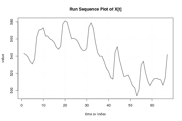
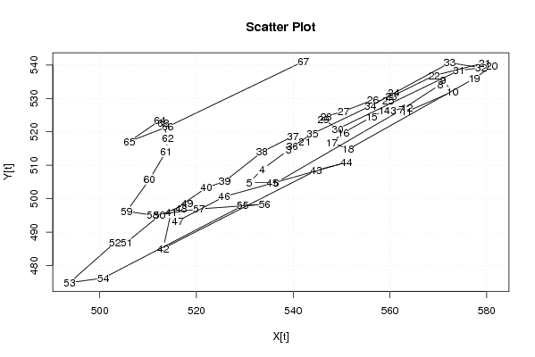
| Dataseries X: | |||||||||||||||||||||||||||||||||||||||||||||||||||||||||||||||||
543,058008 541,7453276 539,031539 533,6065967 530,8653313 536,5202699 562,3726523 570,448946 570,9737297 572,9589863 563,4536361 563,5059893 560,1223081 558,8166068 556,2292693 550,4089389 548,0109488 551,3936888 577,4738089 581,1178882 579,5964113 569,1493653 560,2918882 560,7896219 559,6588246 556,4746176 550,4207482 546,7988661 546,2810632 549,2094318 574,251687 578,8635418 572,3774978 555,984712 543,9816173 539,8268241 539,9462936 533,5522467 525,8089006 522,0785382 514,7630523 513,1179202 544,7990455 550,9972777 535,7182095 525,7632547 516,162765 516,8684552 518,0550164 512,3690076 505,511622 503,1480895 493,7641137 500,7404517 529,5705808 534,0945609 520,5535515 510,9559668 505,5719533 510,2705165 513,7149015 514,0924041 513,1042779 512,4177983 506,1294301 514,0243185 542,0885537 | |||||||||||||||||||||||||||||||||||||||||||||||||||||||||||||||||
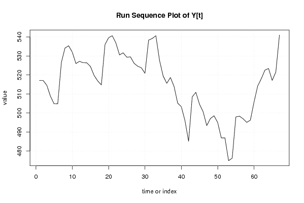
| Dataseries Y: | |||||||||||||||||||||||||||||||||||||||||||||||||||||||||||||||||
517,1199087 517,0744627 514,5648647 508,7858096 504,8207603 504,8445305 526,5614874 534,1825531 535,3522205 532,016917 526,0104562 527,1764411 526,4294825 526,4057371 524,439701 519,7595598 516,8558793 514,774708 535,965484 539,6165305 540,6477596 536,8295819 530,5440604 531,6540228 529,3297649 529,5356456 526,1520693 524,6103316 523,7862159 520,875225 538,3326109 539,1901334 540,6477596 527,7366768 519,4477837 515,617106 518,6848754 513,9805444 505,1712581 503,3418322 496,0413289 485,1515227 508,4840214 510,87474 504,6414569 500,6425871 493,3781511 497,0965701 498,5388651 495,0141412 486,9086157 486,9137501 474,9252573 476,2761804 497,9297139 498,3302118 496,9597569 495,0737319 496,2489295 505,7321425 514,1196359 518,0222003 522,5380369 523,4147495 517,1363457 521,5294814 541,0268016 | |||||||||||||||||||||||||||||||||||||||||||||||||||||||||||||||||
Tables (Output of Computation) | |||||||||||||||||||||||||||||||||||||||||||||||||||||||||||||||||
| |||||||||||||||||||||||||||||||||||||||||||||||||||||||||||||||||
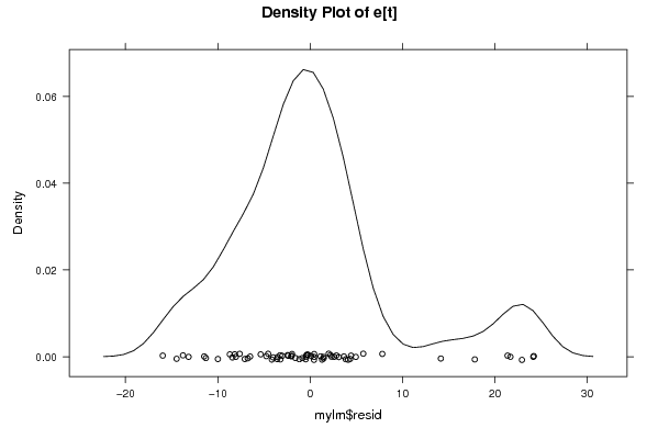
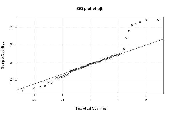
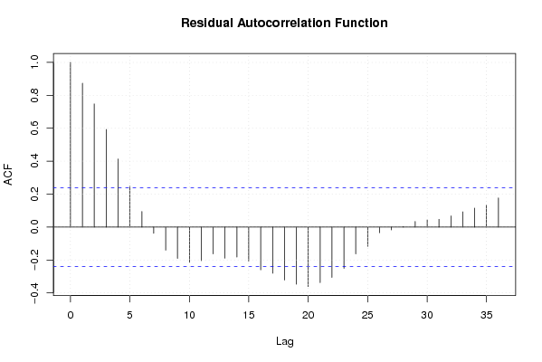
Figures (Output of Computation) | |||||||||||||||||||||||||||||||||||||||||||||||||||||||||||||||||
Input Parameters & R Code | |||||||||||||||||||||||||||||||||||||||||||||||||||||||||||||||||
| Parameters (Session): | |||||||||||||||||||||||||||||||||||||||||||||||||||||||||||||||||
| par1 = 0 ; par2 = 36 ; | |||||||||||||||||||||||||||||||||||||||||||||||||||||||||||||||||
| Parameters (R input): | |||||||||||||||||||||||||||||||||||||||||||||||||||||||||||||||||
| par1 = 0 ; par2 = 36 ; | |||||||||||||||||||||||||||||||||||||||||||||||||||||||||||||||||
| R code (references can be found in the software module): | |||||||||||||||||||||||||||||||||||||||||||||||||||||||||||||||||
par1 <- as.numeric(par1) | |||||||||||||||||||||||||||||||||||||||||||||||||||||||||||||||||